Requirements & scope
Problem Statement & Requirements
Functional Requirements
- Nearby search -- given a user's location (lat, lng) and a radius, return businesses/places sorted by distance and relevance
- Business profiles -- store and serve detailed business information (name, address, hours, photos, menu, categories)
- Search with filters -- filter by category (restaurant, gas station, gym), price range, rating, open now
- Reviews & ratings -- users post reviews and star ratings; aggregate scores displayed
- Business CRUD -- business owners can add, update, and remove their listings
- Photo uploads -- users and owners can upload photos for businesses
- Check-ins -- users can check in at a business (optional social signal)
- Real-time availability -- show open/closed status, wait times, popular hours
- Autocomplete -- suggest businesses and categories as user types (covered in Typeahead design)
Non-Functional Requirements
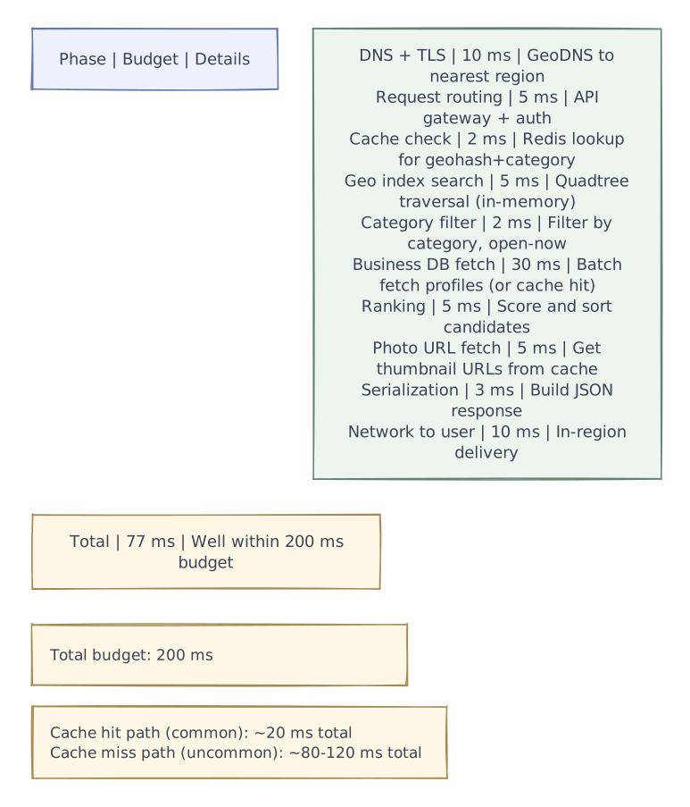
- Low latency -- nearby search results in < 200 ms
- High availability -- 99.99% uptime
- Read-heavy -- read:write ratio ~1000:1 (searches vs. new businesses/reviews)
- Scalability -- 200M businesses, 500M DAU
- Location accuracy -- results accurate to within ~10 meters
- Global coverage -- work everywhere on Earth
- Eventual consistency -- slight delay in new business/review visibility is acceptable
Scope Boundaries
| In Scope | Out of Scope |
|---|---|
| Geospatial indexing & nearby search | Full text search engine (separate system) |
| Business profile storage & serving | Ad platform / sponsored listings (simplified) |
| Review & rating system | Social features (friends, followers) |
| Geohashing, quadtree, R-tree approaches | Turn-by-turn navigation |
| Caching & global serving | Recommendation ML models (simplified) |
| Real-time open/closed status | Reservation / ordering system |
Scale estimations
Scale Estimations
Businesses & Content
| Metric | Value |
|---|---|
| Total businesses worldwide | 200M |
| Average business profile size | 2 KB (text metadata) |
| Average photos per business | 10 |
| Average photo size | 500 KB |
| Total reviews | 5B |
| Average review size | 500 bytes |
| New businesses per day | 100K |
| New reviews per day | 5M |
Traffic
| Metric | Value |
|---|---|
| Daily Active Users (DAU) | 500M |
| Nearby searches per user per day | 5 |
| Total searches per day | 2.5B |
| Searches per second (avg) | ~29K QPS |
| Searches per second (peak) | ~90K QPS |
| Business profile views per day | 1B |
| Profile view QPS | ~12K |
| Write QPS (new businesses + reviews) | ~60 WPS |
| Read:Write ratio | ~1000:1 |
Storage
| Metric | Value |
|---|---|
| Business metadata | 200M × 2 KB = 400 GB |
| Geospatial index (all businesses) | ~20 GB (coordinates + IDs) |
| Reviews | 5B × 500 bytes = 2.5 TB |
| Photos (blob storage) | 200M × 10 × 500 KB = 1 PB |
| User data | 500M × 1 KB = 500 GB |
| Total (excluding photos) | ~3.5 TB |
Geospatial Math
| Metric | Value |
|---|---|
| Earth's surface area | 510M km² |
| Habitable land area | ~150M km² |
| Average business density (urban) | 500-5000 per km² |
| Average business density (overall) | ~1.3 per km² |
| Typical search radius | 1-25 km |
| Businesses in a typical search radius (5 km, urban) | ~40,000 |
Layered architecture
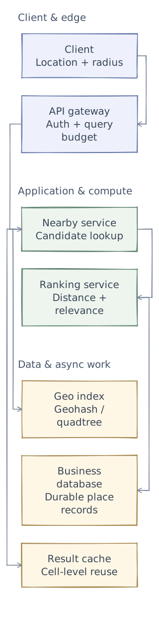
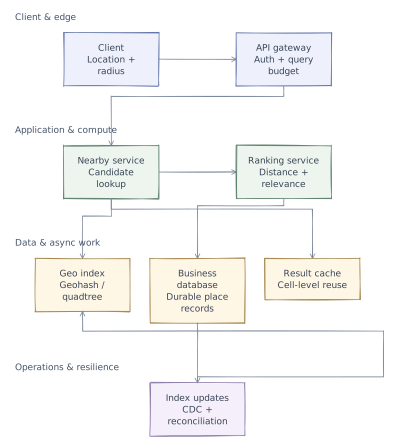
Phase 1 of 4 · Client & edge
Start with the entry points
First, define who uses the system and where requests enter. This is the boundary of the design, not yet a complete request path.
- Client
- Accept a location and bounded search radius; avoid retaining precise location unnecessarily.
- API gateway
- Validate coordinates and cap expensive radius or pagination requests.
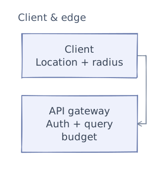
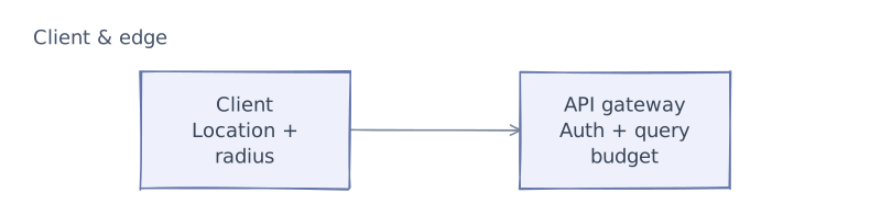
This first layer defines the system boundary. The next chapters add application logic and data dependencies. After examining the request paths and tradeoffs, we will add operational safeguards and bring the complete architecture together.
API & contracts
Phase 2 of 4 · Application & compute
Add the application logic
Keep the entry points and add the services that do the work. Give each service a clear responsibility before defining its contracts. Storage and background dependencies come next.
- Nearby service
- Find spatial cells intersecting the search radius, then filter candidates by exact distance.
- Ranking service
- Combine proximity with business quality and query intent after geographic filtering.
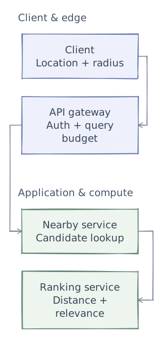
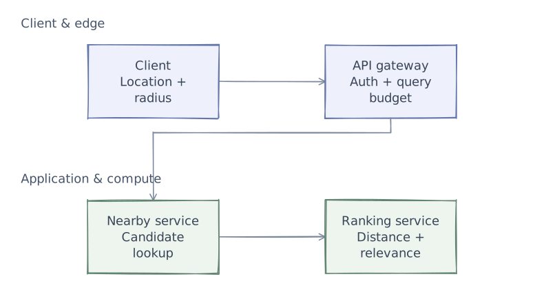
A nearby-search request should specify coordinates, distance units, radius, and filters. Return actual distances rather than presenting cell membership as a distance guarantee. If results depend on changing driver locations or opening hours, declare the freshness expectation and avoid a pagination contract that assumes the candidate set never changes.
Data model
Phase 3 of 4 · Data & async work
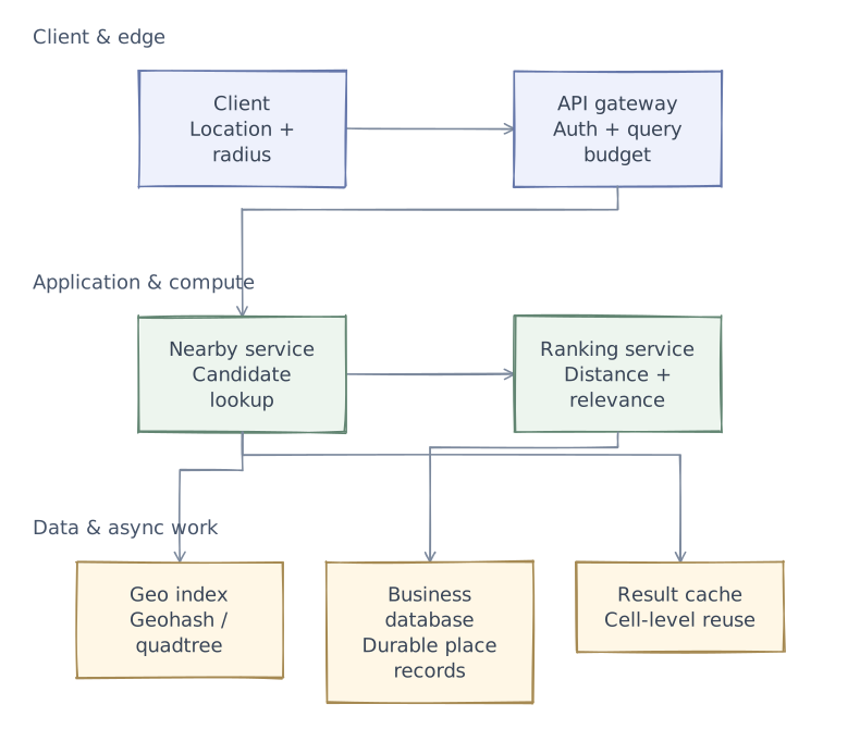
Connect data and background work
The services now need their dependencies: durable state, fast lookups, or work that continues outside a request. Separate these responsibilities rather than treating every component as a database.
- Geo index
- Use a hierarchical spatial index and adjust resolution to local density.
- Business database
- Store business details independently from the rebuildable spatial index.
- Result cache
- Cache reusable cell candidates while preserving freshness for business changes.
Business Data Model & Storage
Database Schema
-- Core business table
CREATE TABLE businesses (
    id              BIGINT PRIMARY KEY AUTO_INCREMENT,
    name            VARCHAR(255) NOT NULL,
    description     TEXT,
    category_id     INT NOT NULL,
    latitude        DECIMAL(10, 7) NOT NULL,
    longitude       DECIMAL(10, 7) NOT NULL,
    geohash         VARCHAR(12) NOT NULL,   -- precomputed geohash
    address         VARCHAR(500),
    city            VARCHAR(100),
    state           VARCHAR(50),
    country         VARCHAR(50),
    zip_code        VARCHAR(20),
    phone           VARCHAR(20),
    website         VARCHAR(500),
    price_range     TINYINT,               -- 1=$, 2=$$, 3=$$$, 4=$$$$
    avg_rating      DECIMAL(2, 1),         -- denormalized, updated async
    review_count    INT DEFAULT 0,         -- denormalized
    is_open         BOOLEAN DEFAULT TRUE,
    owner_id        BIGINT,
    created_at      TIMESTAMP,
    updated_at      TIMESTAMP,

    INDEX idx_geohash (geohash),
    INDEX idx_category_geohash (category_id, geohash),
    INDEX idx_city (city, category_id)
);

-- Business hours
CREATE TABLE business_hours (
    business_id     BIGINT NOT NULL,
    day_of_week     TINYINT NOT NULL,      -- 0=Mon, 6=Sun
    open_time       TIME,
    close_time      TIME,
    is_closed       BOOLEAN DEFAULT FALSE,
    PRIMARY KEY (business_id, day_of_week)
);

-- Categories (hierarchical)
CREATE TABLE categories (
    id              INT PRIMARY KEY,
    name            VARCHAR(100),
    parent_id       INT,                   -- NULL for top-level
    slug            VARCHAR(100),
    INDEX idx_parent (parent_id)
);

-- Reviews
CREATE TABLE reviews (
    id              BIGINT PRIMARY KEY AUTO_INCREMENT,
    business_id     BIGINT NOT NULL,
    user_id         BIGINT NOT NULL,
    rating          TINYINT NOT NULL,      -- 1-5
    text            TEXT,
    photos          JSON,                  -- array of photo URLs
    useful_count    INT DEFAULT 0,
    created_at      TIMESTAMP,

    INDEX idx_business (business_id, created_at DESC),
    INDEX idx_user (user_id, created_at DESC),
    UNIQUE idx_user_biz (user_id, business_id)  -- one review per user per biz
);

-- Photos
CREATE TABLE photos (
    id              BIGINT PRIMARY KEY,
    business_id     BIGINT NOT NULL,
    user_id         BIGINT NOT NULL,
    url             VARCHAR(500),
    caption         VARCHAR(500),
    created_at      TIMESTAMP,
    INDEX idx_business (business_id, created_at DESC)
);
Storage Architecture

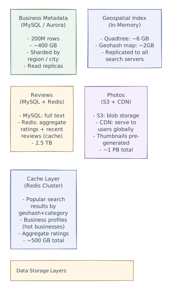
Core design decisions
Geospatial Indexing — Core Approaches
Approach 1: Geohashing

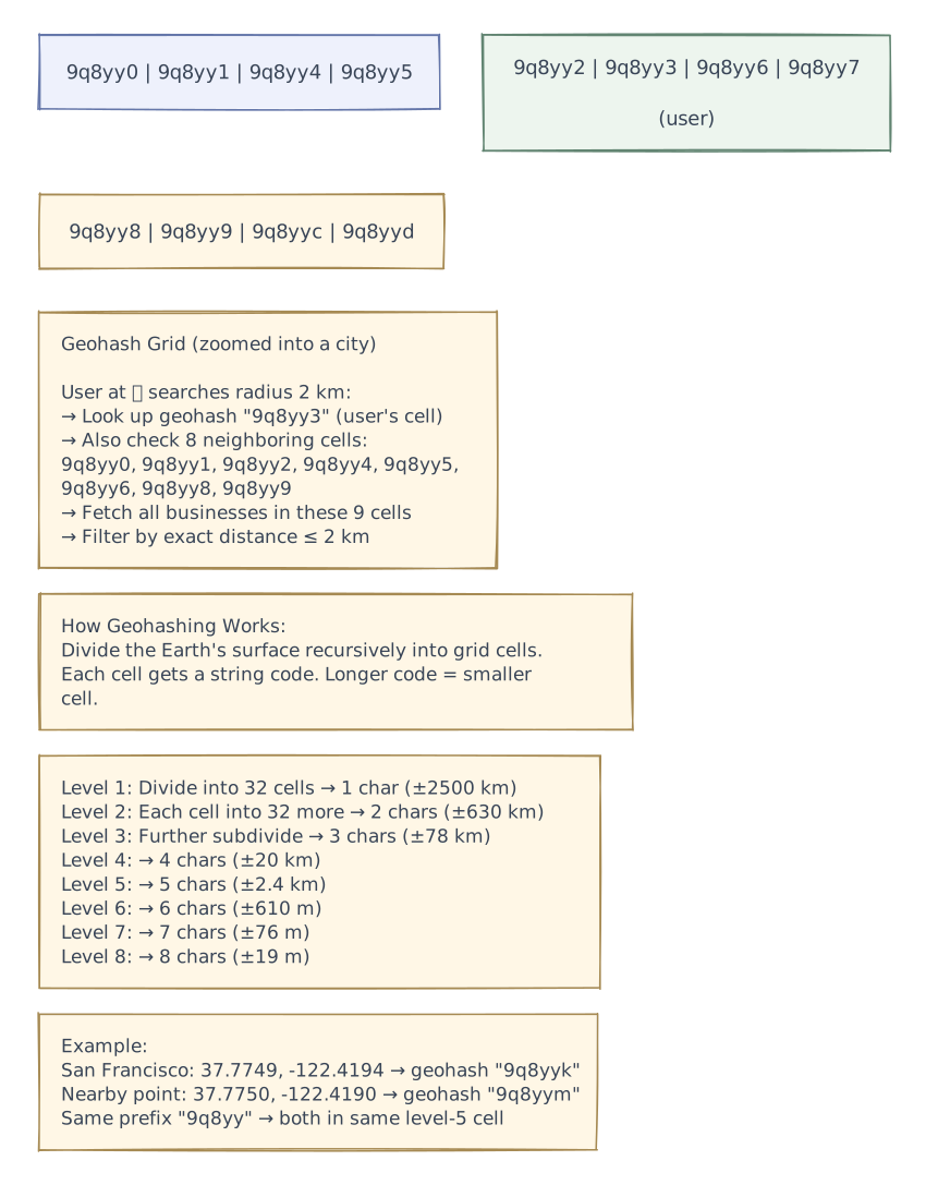
Geohash DB Schema:
CREATE TABLE geo_index (
    geohash     VARCHAR(12),    -- geohash prefix (level 4-6)
    business_id BIGINT,
    latitude    DECIMAL(10, 7),
    longitude   DECIMAL(10, 7),
    PRIMARY KEY (geohash, business_id)
);

-- Index for prefix search:
CREATE INDEX idx_geohash ON geo_index (geohash);

-- Query: Find businesses near (37.7749, -122.4194) within 2 km
-- Step 1: Compute geohash at level 5: "9q8yy"
-- Step 2: Find 8 neighbors: "9q8yz", "9q8yv", ...
-- Step 3:
SELECT business_id, latitude, longitude
FROM geo_index
WHERE geohash IN ('9q8yy', '9q8yz', '9q8yv', '9q8yw',
                   '9q8yx', '9q8yt', '9q8ys', '9q8ym', '9q8yq')
-- Step 4: Post-filter by haversine distance ≤ 2 km
Geohash Pros & Cons:
| Pros | Cons |
|---|---|
| Simple to implement (string prefix) | Edge problem: nearby points across cell boundary have very different geohashes |
| Works with any DB (just string prefix queries) | Fixed grid — can't adapt to density variations |
| Easy to cache (geohash → businesses) | Must check 9 cells (center + 8 neighbors) to handle boundaries |
| Composable with other indexes | Precision levels are discrete jumps, not continuous radius |
Approach 2: Quadtree
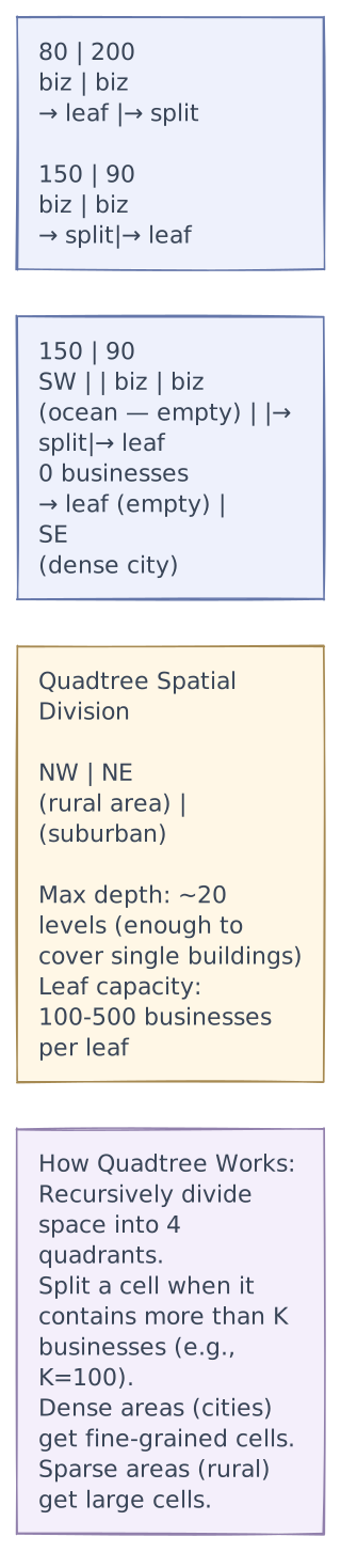
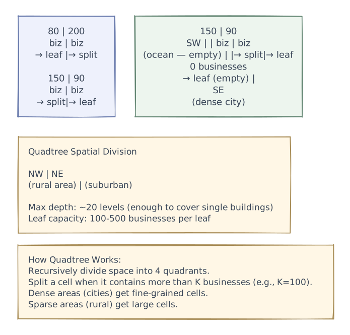
Quadtree Node Structure:
struct QuadTreeNode {
    // Bounding box for this node
    top_left: (f64, f64),       // (lat, lng)
    bottom_right: (f64, f64),   // (lat, lng)

    // Leaf node: contains businesses
    businesses: Vec<BusinessId>, // up to capacity K

    // Internal node: 4 children
    nw: Option<Box<QuadTreeNode>>,
    ne: Option<Box<QuadTreeNode>>,
    sw: Option<Box<QuadTreeNode>>,
    se: Option<Box<QuadTreeNode>>,

    // Metadata
    count: u32,  // total businesses in subtree
}

Memory per internal node: ~100 bytes (pointers + bounds)
Memory per leaf node: ~100 bytes + K × 8 bytes (business IDs)

For 200M businesses, K=100:
  Leaf nodes: 200M / 100 = 2M leaves
  Internal nodes: ~2M / 3 ≈ 700K
  Total nodes: ~2.7M
  Memory: 2.7M × 200 bytes = ~540 MB
  With business coordinates: + 200M × 24 bytes = ~4.8 GB
  Total in-memory quadtree: ~5-6 GB
Quadtree Search Algorithm:
search(node, center, radius):
    if node does not intersect circle(center, radius):
        return []  // prune this subtree

    if node is leaf:
        return [b for b in node.businesses
                if distance(b.location, center) ≤ radius]

    results = []
    for child in [node.nw, node.ne, node.sw, node.se]:
        if child is not None:
            results.extend(search(child, center, radius))
    return results

Time complexity: O(K + number_of_visited_nodes)
  Visited nodes: depends on how many cells the search circle overlaps
  Typical: 10-50 nodes for a 5 km radius search
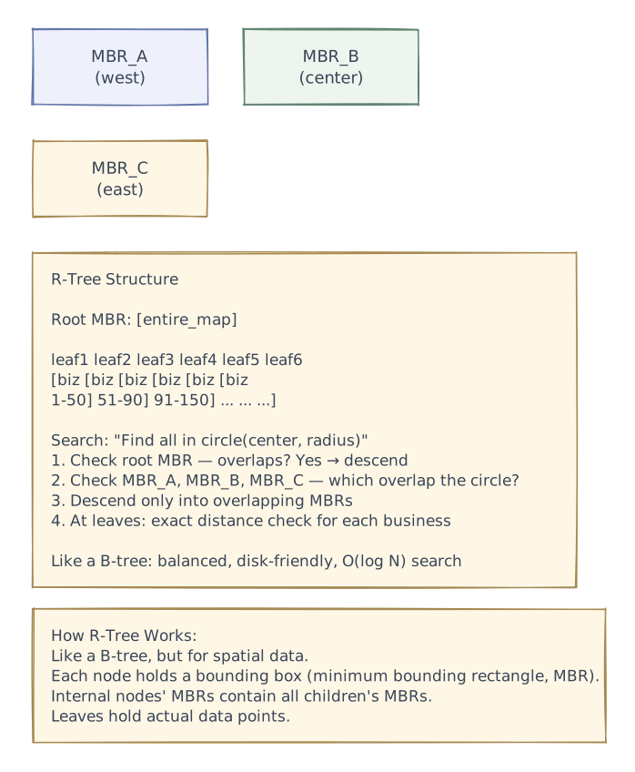
Approach 3: R-Tree

Comparison of Geospatial Indexes
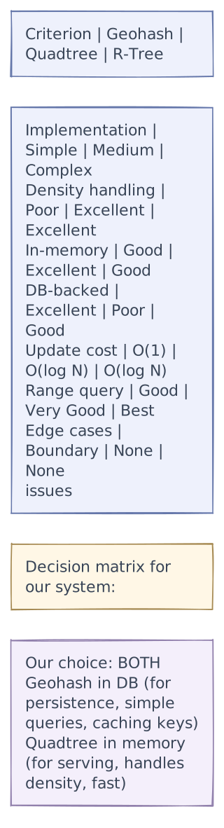
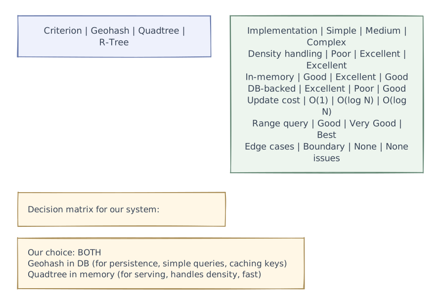
| Criterion | Geohash | Quadtree | R-Tree |
|---|---|---|---|
| Complexity | Simple (string ops) | Medium | High |
| Adaptivity | Fixed grid (non-adaptive) | Adaptive to density | Adaptive to density |
| Memory | Low (~2 GB for 200M points) | Medium (~5 GB) | Medium (~5 GB) |
| Search efficiency | Good (9-cell lookup) | Very good (prune empty regions) | Best (balanced, minimal overlap) |
| Update cost | O(1) — just insert row | O(log N) — may trigger split | O(log N) — may trigger rebalance |
| Edge cases | Cross-boundary issues | None | None |
| DB support | Any DB (string prefix) | Custom in-memory | PostGIS, MongoDB, many DBs |
| Best for | Simple systems, DB-backed | In-memory serving, variable density | Disk-backed, complex queries |
| Used by | Elasticsearch, Redis | Uber H3 (variant), custom | PostGIS, MongoDB, Oracle Spatial |
Our choice: Geohash for DB storage + In-memory Quadtree for serving
- Geohash in the database for persistence and simple queries
- In-memory Quadtree in the search service for low-latency serving
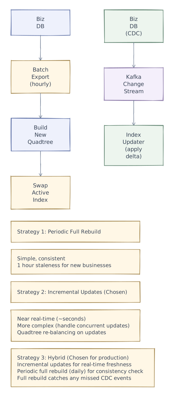
- Quadtree rebuilt from DB periodically or updated incrementally
Ranking & Relevance
Scoring Formula
For each candidate business within the search radius:

score(business, query) =
    w_dist  × distance_score(business, user_location)
  + w_rate  × rating_score(business)
  + w_rev   × review_count_score(business)
  + w_rel   × category_relevance(business, query)
  + w_open  × is_open_now_boost(business)
  + w_price × price_match(business, query)
  + w_pop   × popularity_score(business)

Where:
  distance_score = 1 - (distance / max_radius)     -- closer = higher
  rating_score   = avg_rating / 5.0                 -- normalized to [0, 1]
  review_count_score = log(review_count + 1) / log(max_reviews + 1)
  is_open_now_boost  = 1.0 if open, 0.3 if closed
  popularity_score   = log(recent_views + recent_checkins + 1) / normalization_factor

Default weights:
  w_dist  = 0.30    -- distance is most important
  w_rate  = 0.25    -- rating is second
  w_rev   = 0.15    -- review count (social proof)
  w_rel   = 0.10    -- category match
  w_open  = 0.10    -- open now bias
  w_price = 0.05    -- price preference
  w_pop   = 0.05    -- popularity

Weights adjusted by context:
  - "best restaurants" → increase w_rate to 0.40
  - "nearest gas station" → increase w_dist to 0.50
  - "cheap eats" → increase w_price to 0.15
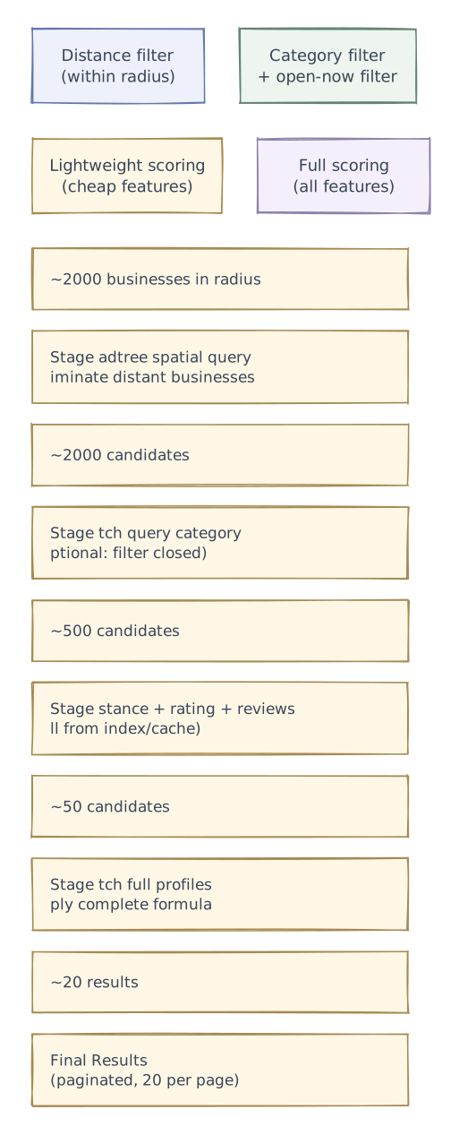
Ranking Pipeline

Request flows
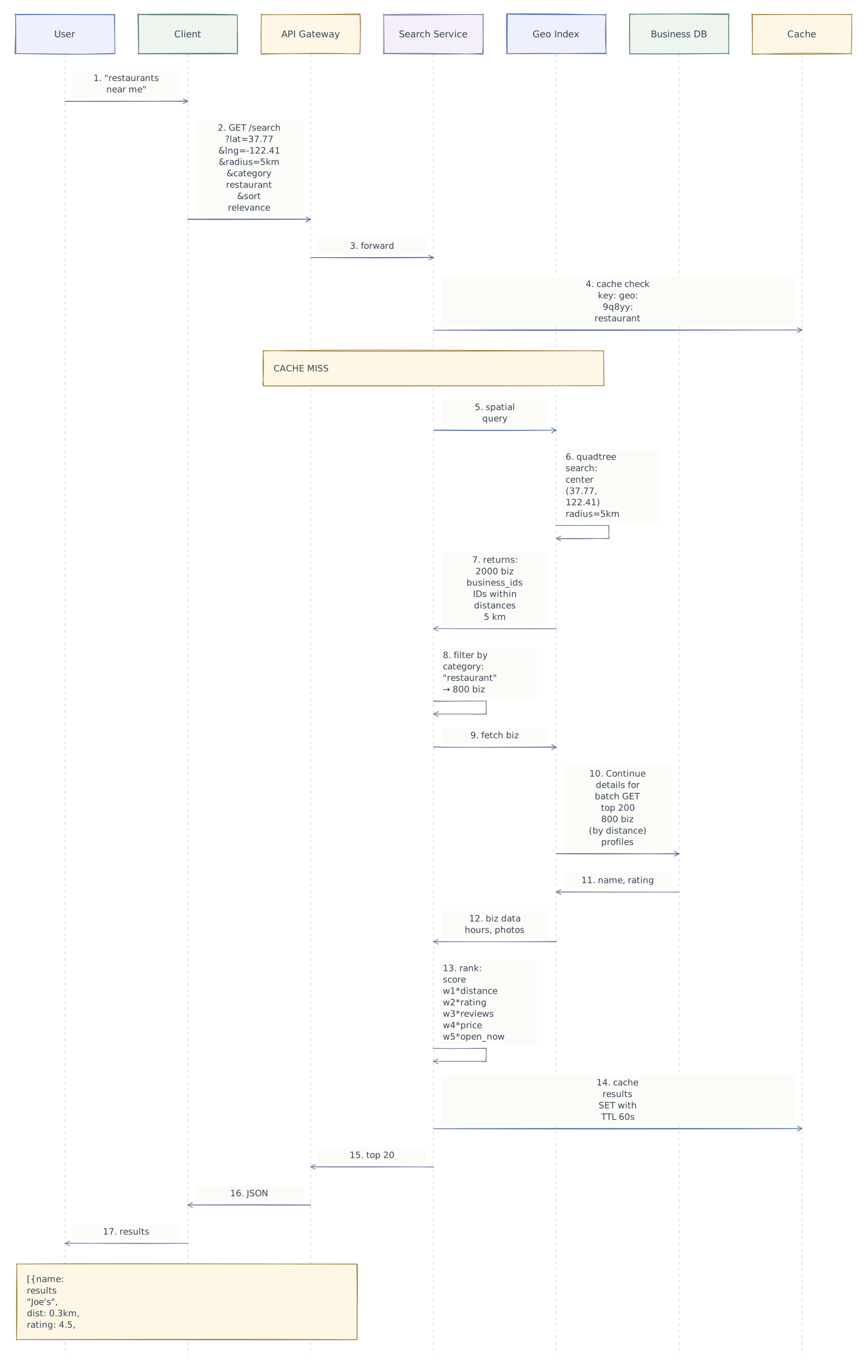
Nearby Search Flow
End-to-End Search Flow

Distance Calculation
Haversine Formula (great-circle distance on a sphere):

d = 2R × arcsin(√(sin²(Δlat/2) + cos(lat1) × cos(lat2) × sin²(Δlng/2)))

Where:
  R = 6,371 km (Earth's radius)
  lat1, lat2 = latitudes in radians
  lng1, lng2 = longitudes in radians
  Δlat = lat2 - lat1
  Δlng = lng2 - lng1

Optimization for ranking (avoid expensive trig):
  Use squared Euclidean distance on projected coordinates
  for APPROXIMATE ranking within small areas (< 50 km):

  dx = (lng2 - lng1) × cos(lat_center)  // longitude degrees → km factor
  dy = lat2 - lat1
  approx_distance² = dx² + dy²

  Only compute exact haversine for final top-K results
and for boundary filtering (is distance ≤ radius?)Performance & caching
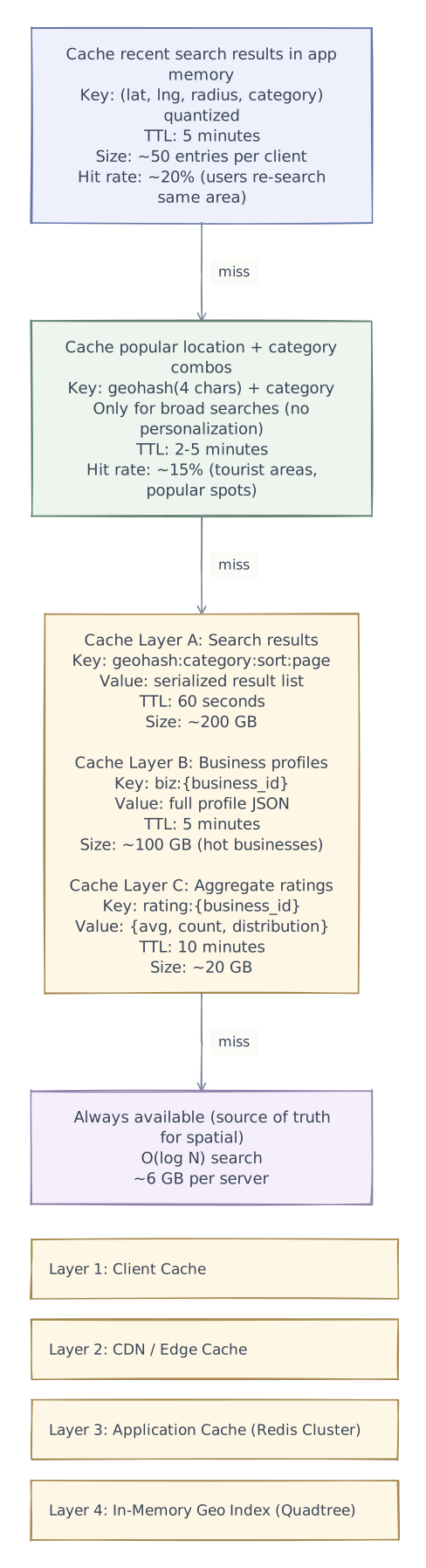
Caching Strategy
Multi-Layer Cache

Cache Key Design for Geospatial Queries
Problem: Exact (lat, lng) pairs almost never repeat.
         Caching by exact coordinates → 0% hit rate.

Solution: Quantize location to geohash cell.

  User at (37.77491, -122.41943) → geohash level 5: "9q8yy"
  User at (37.77512, -122.41900) → geohash level 5: "9q8yy"  (same!)

  Cache key: "search:9q8yy:restaurant:rating_desc:page1"

  All users in the same ~2.4 km × 2.4 km cell share the same cache.
  In a dense area, this covers ~500 meters for level-6 geohash.

  Tradeoff: quantization level
    Level 4 (20 km cell): Higher hit rate, less precise
    Level 5 (2.4 km cell): Good balance ← chosen
    Level 6 (610 m cell): Lower hit rate, more precise

  The search service still computes exact distances for ranking,
but the candidate set (from geo index) is cached at geohash granularity.Advanced design
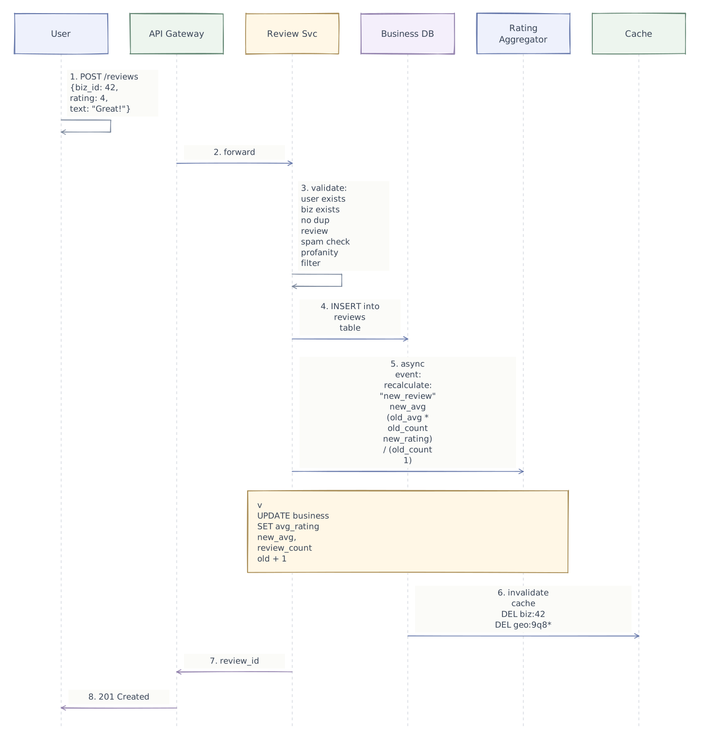
Review & Rating System
Review Submission Flow

Rating Aggregation Strategies
Approach 1: Simple Average
  avg_rating = SUM(rating) / COUNT(ratings)
  Problem: A business with 1 review of 5.0 ranks above
           a business with 1000 reviews averaging 4.8

Approach 2: Bayesian Average (Chosen)
  bayesian_avg = (C × m + Σ ratings) / (C + n)

  Where:
    n = number of reviews for this business
    m = global average rating across all businesses (~3.7)
    C = confidence parameter (typically 10-50)

  Example:
    Business A: 1 review, 5.0 stars
      bayesian = (10 × 3.7 + 5.0) / (10 + 1) = 3.82

    Business B: 1000 reviews, 4.8 avg
      bayesian = (10 × 3.7 + 4800) / (10 + 1000) = 4.79

  Business B correctly ranks higher.

Approach 3: Time-Weighted Average
  Recent reviews matter more:
  weighted_avg = Σ (rating_i × decay(age_i)) / Σ decay(age_i)
  decay(age) = e^(-λ × age_in_days), λ = 0.01

  Captures improving or declining businesses.
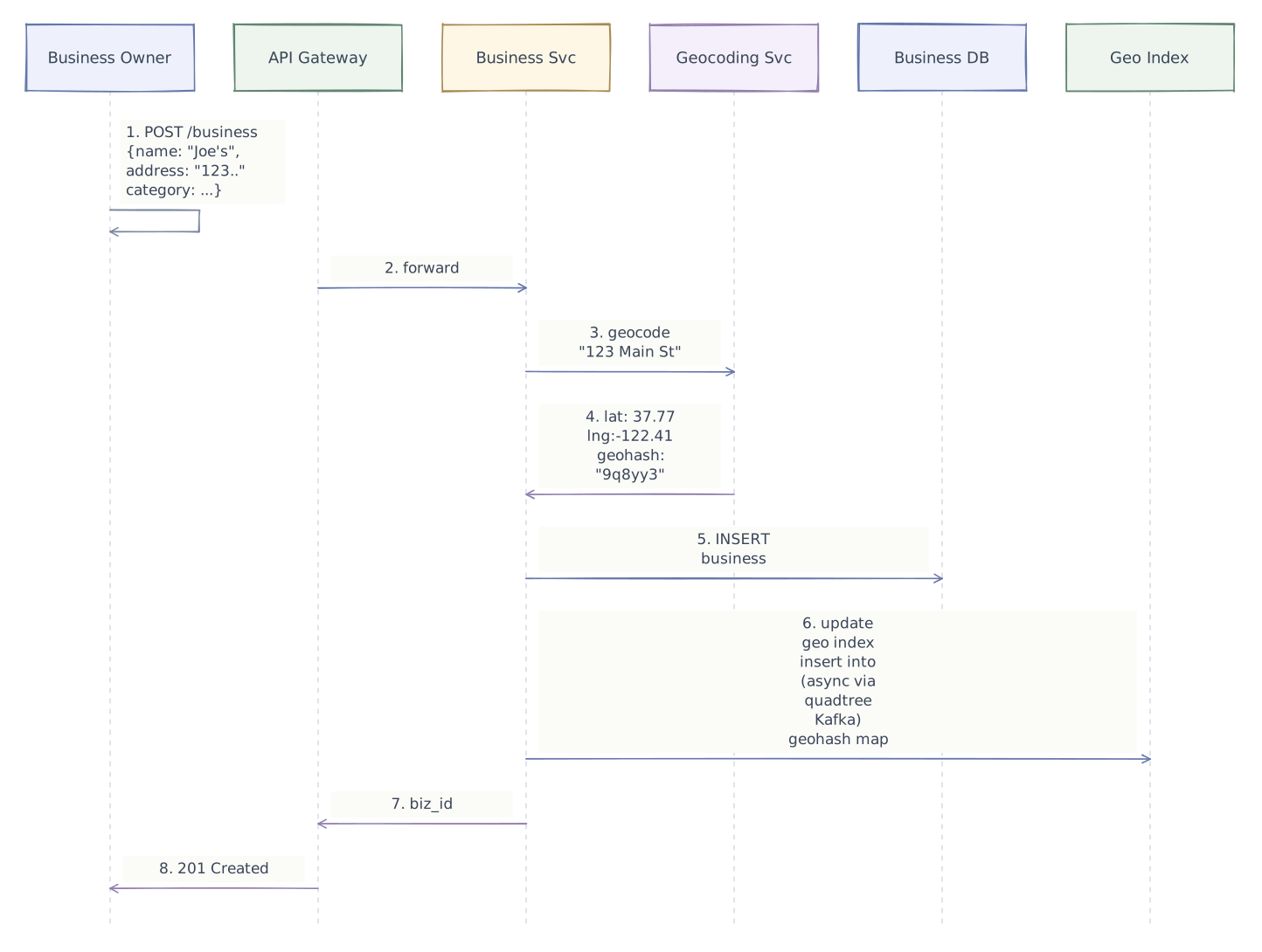
Business Update & Index Sync
Write Path: Adding / Updating a Business

Index Synchronization Strategies

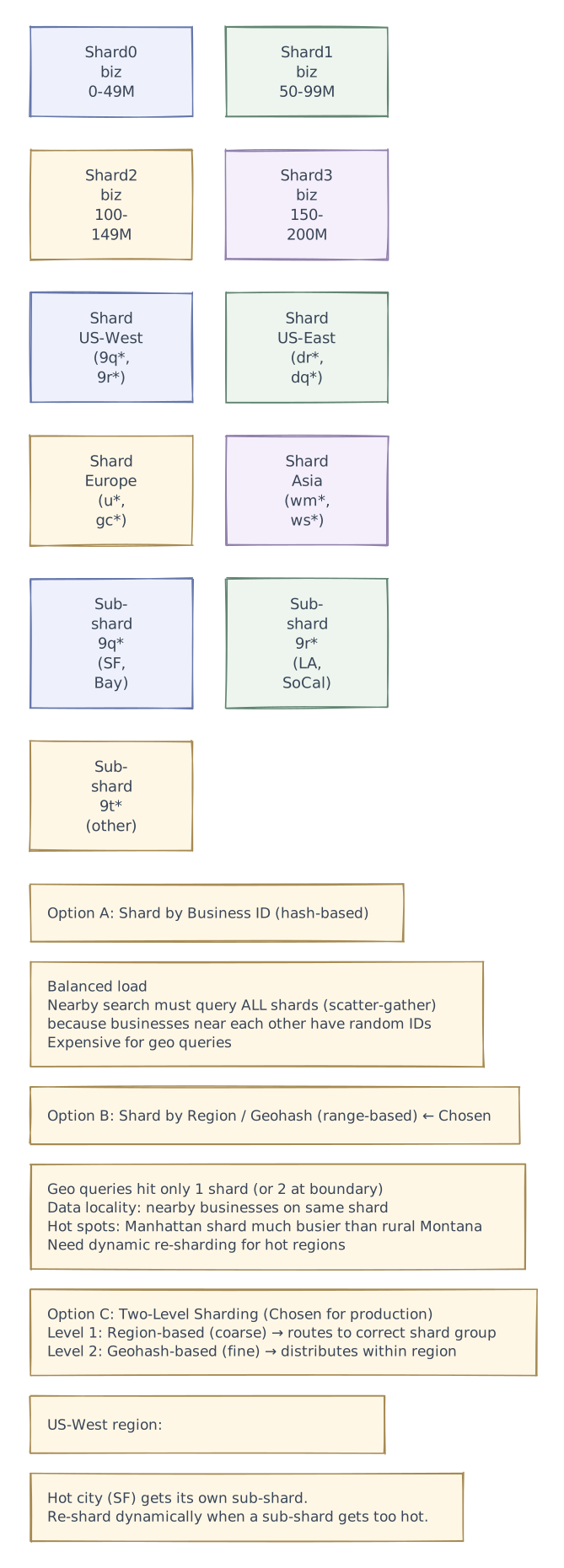
Sharding Strategy
Business Database Sharding

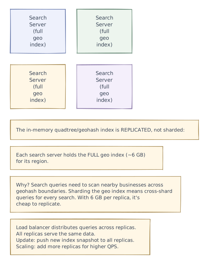
Geo Index Replication

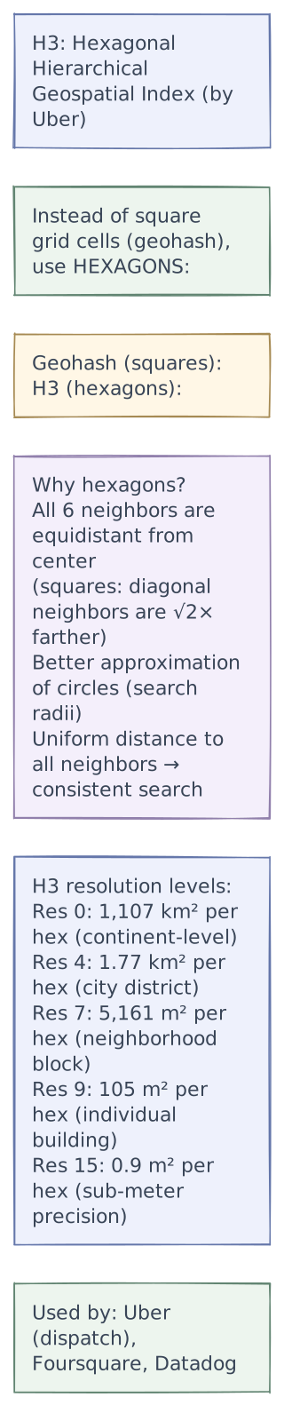
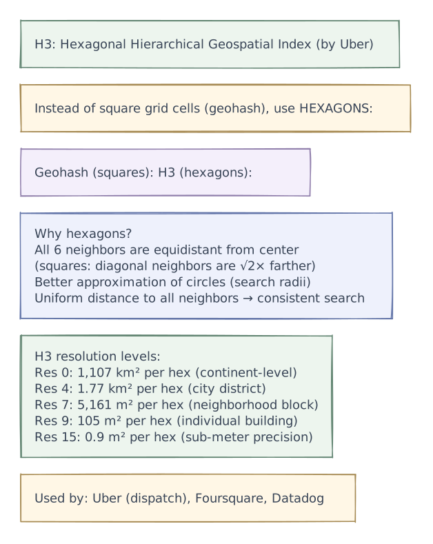
Uber H3: Modern Alternative to Geohash
Edge cases
Handling Density Variations
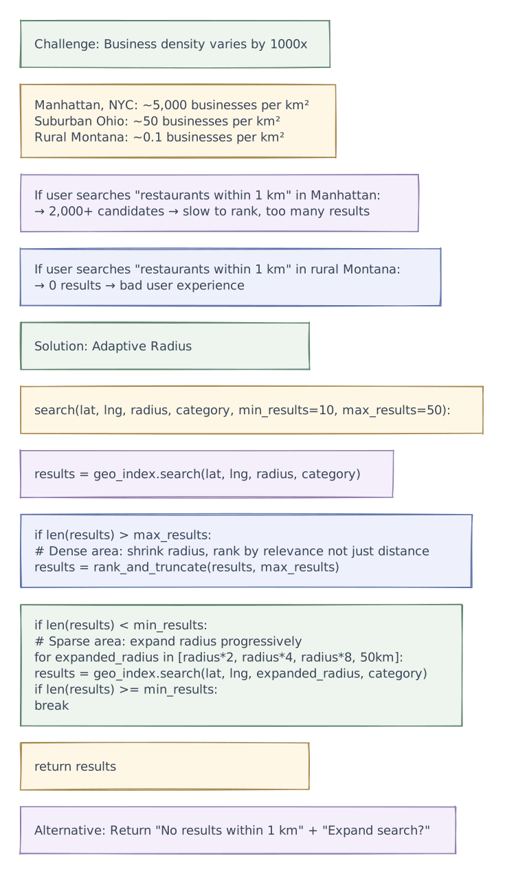
The Density Problem

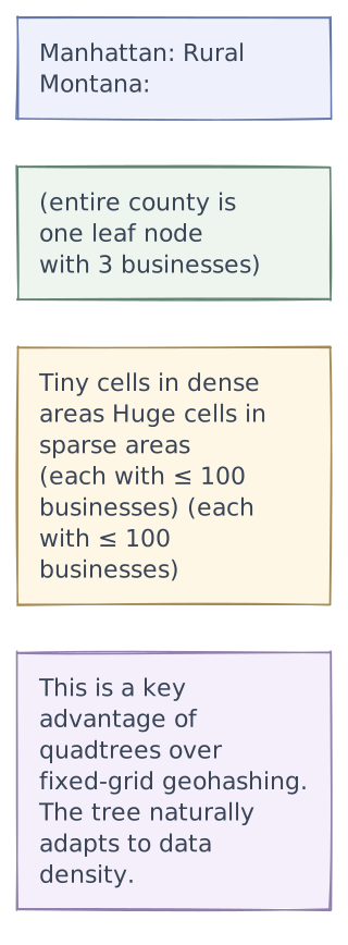
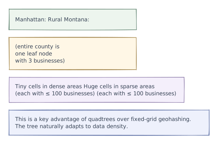
Quadtree Handles Density Naturally
Tradeoffs
Key Tradeoffs
Geohash vs. Quadtree vs. R-Tree
Pre-Computed Results vs. On-the-Fly
Pre-computed (for popular locations/categories):
  + Instant response (cache hit)
  + Offload computation from serving path
  - Stale results (TTL-dependent)
  - Storage cost for all location × category combinations
  - Can't personalize pre-computed results

On-the-fly (for long-tail queries):
  + Always fresh
  + Can personalize (user preferences, history)
  - Higher latency (geo search + DB fetch + ranking)
  - Higher compute cost per query

Hybrid (chosen):
  - Pre-compute results for top 1000 geohash cells × top 20 categories
    = 20,000 cached result sets (updated every 60 seconds)
  - On-the-fly for everything else (long-tail locations, complex filters)
  - Cache on-the-fly results with TTL for reuse
Read Replicas vs. Denormalization
Problem: Search results need business name, rating, review count,
         hours, photos — all from different tables.

Option A: Join at query time (read replicas)
  SELECT b.*, AVG(r.rating), COUNT(r.id), ...
  FROM businesses b
  JOIN reviews r ON b.id = r.business_id
  WHERE b.id IN (id1, id2, ..., id200)
  GROUP BY b.id

  + Always consistent
  - Expensive joins at query time
  - Latency: ~50-100 ms for 200 businesses

Option B: Denormalize into business table (chosen)
  businesses table includes:
    avg_rating (updated async on new review)
    review_count (updated async on new review)
    primary_photo_url (updated async on new photo)
    next_open_time (updated periodically)

  Query: simple SELECT * FROM businesses WHERE id IN (...)
  Latency: ~5-10 ms for 200 businesses

  + Fast reads
  - Slight staleness (async updates)
  - Must maintain consistency between tables

Tradeoff: Acceptable for our use case.
  A review posted 5 seconds ago not immediately reflected
  in avg_rating is fine (eventual consistency).
Proximity Sort vs. Relevance Sort
User expectation varies by query:

"gas station near me" → DISTANCE is primary
  - User needs the nearest one, quality doesn't matter
  - Sort by distance, minimal relevance scoring

"best sushi restaurant" → RELEVANCE is primary
  - User wants quality, willing to travel further
  - Sort by rating × distance blend

"pizza" → BALANCED
  - User wants good pizza that's not too far
  - Default: 60% distance, 40% quality

Implementation:
  sort_mode = infer_from_query(query)
  if "near" or "nearby" or "closest" in query:
      sort_mode = DISTANCE_FIRST
  elif "best" or "top" in query:
      sort_mode = RELEVANCE_FIRST
  else:
      sort_mode = BALANCED

  Adjust ranking weights accordingly.
Static Index vs. Dynamic Index
Static (rebuild periodically):
  + Consistent, optimized data structure
  + No concurrent modification issues
  + Can apply global optimizations (rebalance quadtree)
  - Stale for new businesses (up to rebuild interval)
  - Full rebuild is expensive (200M businesses)

Dynamic (update in real-time):
  + Immediately reflects new/updated businesses
  + No rebuild downtime
  - Concurrent read/write complexity
  - Gradual degradation (unbalanced quadtree)
  - Memory fragmentation over time

Chosen: Dynamic with periodic rebalance
  - Incremental updates via CDC (seconds latency)
  - Full rebuild daily (off-peak) for rebalancing
- Blue/green swap for zero-downtime rebuildsReliability & fault tolerance
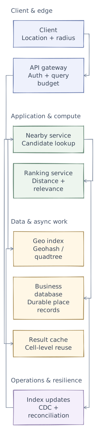
Phase 4 of 4 · Operations & resilience
Add operational safeguards
With the request paths and tradeoffs established, add the controls that help detect trouble and keep the system operating. The final diagram retains every layer introduced so far.
- Index updates
- Propagate location and listing changes and detect divergence between the index and database.
Fault Tolerance & Reliability
Failure Scenarios & Handling
| Failure | Impact | Mitigation |
|---|---|---|
| Search server crash | One replica unavailable | Load balancer routes to other replicas; auto-restart |
| Geo index corruption | Wrong/missing search results | Rebuild from DB; checksum validation on load |
| Business DB primary fails | Writes fail | Promote read replica to primary (automated failover) |
| Redis cache cluster down | Higher load on DB | Business DB read replicas absorb load; degraded latency |
| Photo CDN outage | Missing thumbnails | Serve placeholder images; fallback to origin |
| Geocoding service down | Can't add new businesses | Queue new business submissions; process when restored |
| Kafka lag (CDC events) | Stale geo index | Alert; fallback to periodic full rebuild |
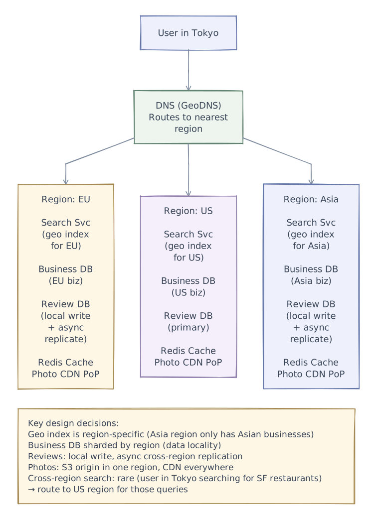
| Entire region down | Users in region can't search | DNS failover to next-nearest region |
Graceful Degradation
When system is under stress:

Level 1: Reduce ranking quality
  - Skip ML-based ranking → use simple distance + rating formula
  - Save ~20 ms per query

Level 2: Increase cache TTL
  - Extend from 60s to 5 min
  - Serve slightly stale results
  - Dramatically reduce DB load

Level 3: Reduce candidate set
  - Return 10 results instead of 20
  - Search smaller radius
  - Skip "expand radius" for sparse areas

Level 4: Return cached-only results
  - Only serve queries with cache hits
  - Return "service busy" for cache misses
  - Last resort before complete outage
Monitoring & Operational Concerns
Key Metrics
| Category | Metric | Alert Threshold |
|---|---|---|
| Latency | P50 search latency | > 50 ms |
| Latency | P99 search latency | > 300 ms |
| Availability | Search success rate | < 99.9% |
| Quality | Avg results per search | < 5 (too few) |
| Quality | "No results" rate | > 2% |
| Freshness | New business indexing delay | > 5 min |
| Freshness | Review aggregation delay | > 2 min |
| Cache | Redis hit rate | < 60% |
| Index | Quadtree node count | > 5M (unexpected growth) |
| Index | Geo index memory usage | > 8 GB per server |
| DB | Read replica lag | > 5 seconds |
Production architecture
High-Level Architecture

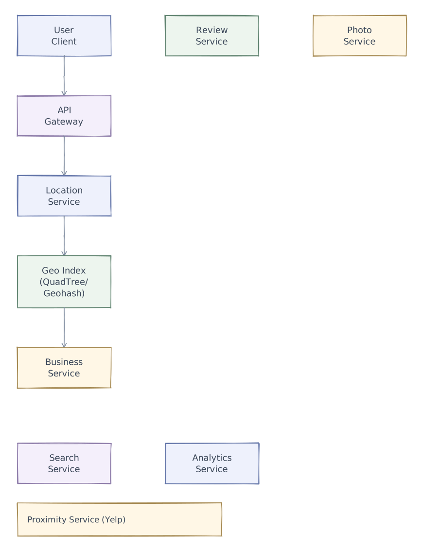
Detailed Architecture

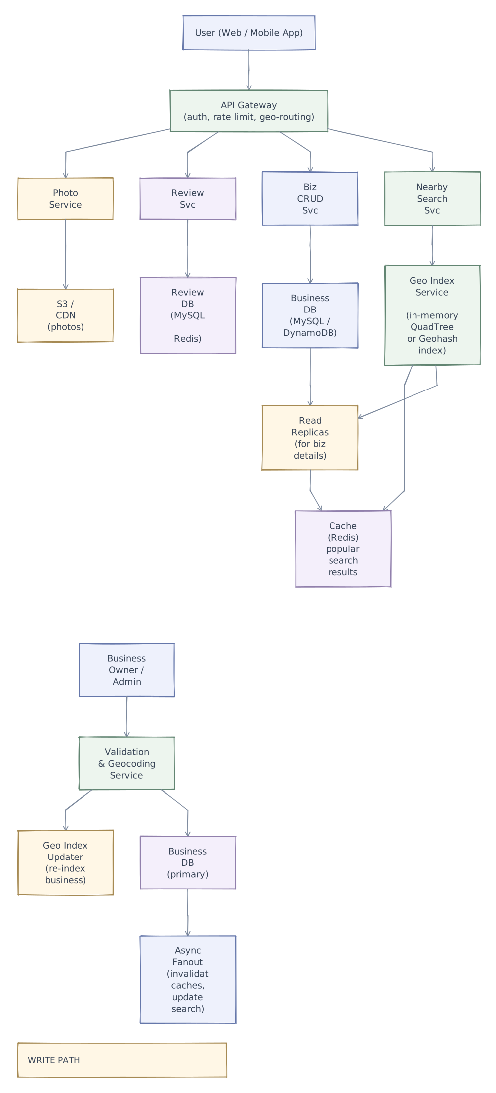
Global Deployment
Multi-Region Architecture

Latency Budget
Further exploration
Advanced Features
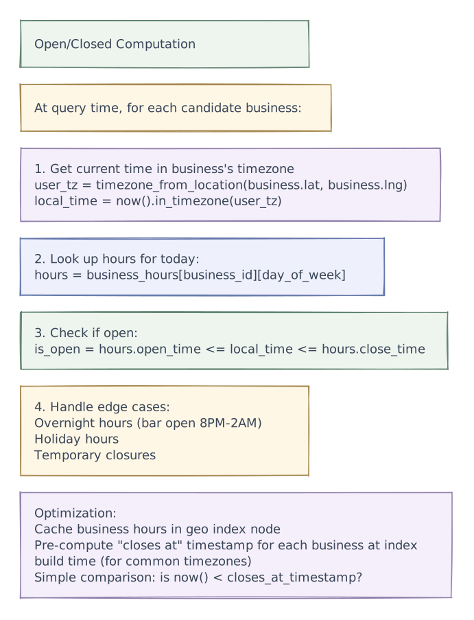
Real-Time Open/Closed Status

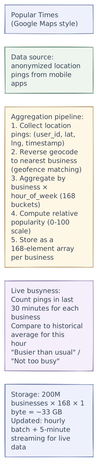
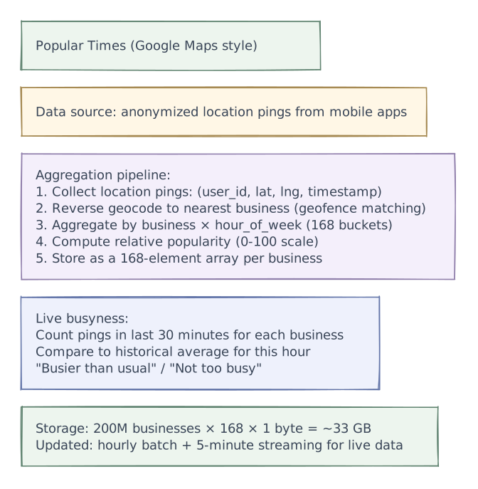
Popular Times / Wait Times
Map Tile Clustering
When showing businesses on a map at low zoom levels,
individual pins overlap → cluster them:

Zoom level 15 (street):     Zoom level 12 (city):
  🍕 🍔 🍜                    (42) 🍕🍔🍜🍣...
  🍣 🍕 🏪                    clustered into one icon
  🍔 🍜 🍕                    showing count

Clustering algorithm (server-side):
  1. Determine visible map bounds (lat/lng bounding box)
  2. Determine zoom level → grid cell size
  3. Assign each business to a grid cell
  4. For each cell with > 1 business:
     - Create cluster: center = centroid, count = N
  5. Return clusters + individual pins

Implementation:
  Use geohash at appropriate precision for zoom level:
    Zoom 5  → geohash length 2 (large clusters)
    Zoom 10 → geohash length 4 (medium clusters)
    Zoom 15 → geohash length 6 (individual pins)

GROUP BY geohash_prefix → instant clusteringInterview playbook
System Design Interview Tips
What Interviewers Look For
- Geospatial indexing -- can you explain geohash vs quadtree vs R-tree and when to use each?
- Scale reasoning -- 200M businesses, 30K QPS, how much memory for the index?
- Two-phase search -- spatial filter (geo index) → business lookup (DB) → ranking
- Caching by geohash -- key insight for making geo queries cacheable
- Density handling -- adaptive radius, quadtree's natural density adaptation
- Tradeoff reasoning -- geohash vs quadtree, static vs dynamic index, precision vs recall
Common Follow-Up Questions
| Question | Key Points |
|---|---|
| "How do you handle the geohash boundary problem?" | Check center cell + 8 neighbors; or use quadtree (no boundary issues) |
| "What if someone searches across a region boundary?" | Route to the region that contains most of the search radius; or fan-out to 2 regions |
| "How do you keep ratings fresh?" | Async aggregation on review write; denormalize into business table; cache with short TTL |
| "How would you add 'reserve a table' feature?" | Separate reservation service; business profile links to availability API |
| "How do you handle a business with multiple locations?" | Each location is a separate business entity in the DB; chain_id links them |
| "What about privacy for popular times data?" | Anonymize + aggregate; k-anonymity (don't report if < K users in a cell); differential privacy |
Suggested 45-Minute Interview Structure
 0-5  min:  Clarify requirements (nearby search? reviews? scale?)
 5-10 min:  Scale estimations (businesses, QPS, storage, memory)
10-20 min:  Geospatial indexing deep dive (geohash + quadtree)
20-30 min:  System architecture (search flow, DB schema, caching)
30-38 min:  Deep dive: pick ONE
            - Option A: Ranking & relevance scoring
            - Option B: Sharding & global deployment
            - Option C: Review & rating aggregation
38-43 min:  Tradeoffs (geohash vs quadtree, static vs dynamic, density handling)
43-45 min:  Monitoring, failure handling, extensions