Requirements & scope
Problem Statement & Requirements
Functional Requirements
- Personalized recommendations -- show items (products, videos, songs, articles) tailored to each user's interests
- Multiple surfaces -- home feed, "similar items", "customers also bought", "because you watched X"
- Real-time signals -- incorporate recent user actions (clicks, purchases, watches) within seconds
- Multi-modal content -- recommend across content types (videos + articles, products + accessories)
- Explanation -- provide reason for recommendation ("Because you liked X", "Trending in your area")
- Diversity & freshness -- avoid echo chambers; mix in new/diverse items alongside safe bets
- Cold start -- handle new users (no history) and new items (no interactions)
- Negative feedback -- "Not interested" / "Don't recommend" signals respected immediately
- Contextual awareness -- time of day, device, location influence recommendations
Non-Functional Requirements
- Low latency -- recommendations rendered in < 200 ms
- High availability -- 99.99% uptime; fallback to popular/trending if personalization fails
- Massive scale -- 500M users, 100M items, 10B+ interactions per day
- Freshness -- new items discoverable within minutes; user actions reflected within seconds
- Offline efficiency -- model training on petabytes of interaction data within hours
- A/B testable -- run multiple recommendation models simultaneously for experimentation
Scope Boundaries
| In Scope | Out of Scope |
|---|---|
| Candidate generation (retrieval) | Full search engine (covered separately) |
| Ranking / scoring | Ad auction system |
| Embedding models (two-tower, matrix factorization) | Detailed NLP / LLM integration |
| Feature store & serving | Data warehouse infrastructure |
| A/B testing framework (simplified) | Full experimentation platform |
| Cold start strategies | Content moderation / safety filtering (simplified) |
Scale estimations
Scale Estimations
Users & Items
| Metric | Value |
|---|---|
| Total users | 1B |
| Daily Active Users (DAU) | 500M |
| Total items (catalog) | 100M |
| New items per day | 500K |
| Average interactions per user per day | 20 (views, clicks, purchases) |
| Total interactions per day | 10B |
| Historical interactions (1 year) | 3.6T |
Traffic
| Metric | Value |
|---|---|
| Recommendation requests per day | 5B (10 per user per day) |
| Requests per second (avg) | ~58K RPS |
| Requests per second (peak) | ~150K RPS |
| Items scored per request | ~1000 (after retrieval, before final ranking) |
| Embedding lookups per request | ~100-500 (ANN retrieval) |
Storage
| Metric | Value |
|---|---|
| User embedding vectors (500M × 256 dims × 4 bytes) | ~500 GB |
| Item embedding vectors (100M × 256 dims × 4 bytes) | ~100 GB |
| Interaction logs (1 year, compressed) | ~50 TB |
| Feature store (user + item features) | ~2 TB |
| User-item interaction matrix (sparse) | ~10 TB |
| Model artifacts (all versions) | ~500 GB |
Compute
| Metric | Value |
|---|---|
| Model training (daily) | 1000s of GPUs, ~4-8 hours |
| Embedding index (ANN) | ~100 GB in memory per replica |
| Feature store serving | ~2 TB across Redis cluster |
| Ranking inference | ~1 ms per candidate (batch of 1000 = ~50 ms with GPU) |
Layered architecture
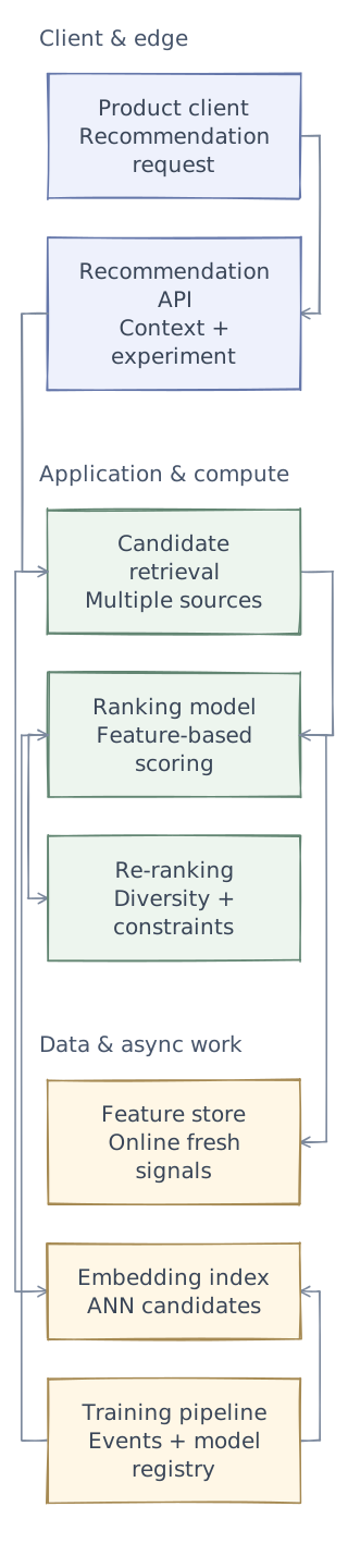
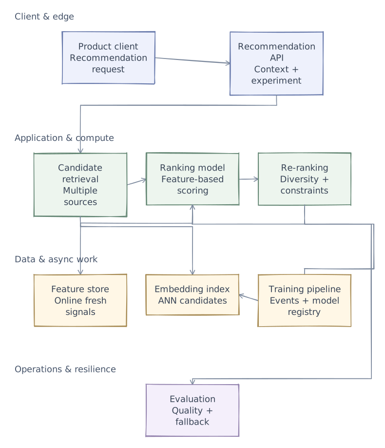
Phase 1 of 4 · Client & edge
Start with the entry points
First, define who uses the system and where requests enter. This is the boundary of the design, not yet a complete request path.
- Product client
- Define the recommendation surface and its latency budget before selecting models.
- Recommendation API
- Attach request context and a stable experiment assignment.
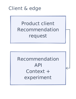
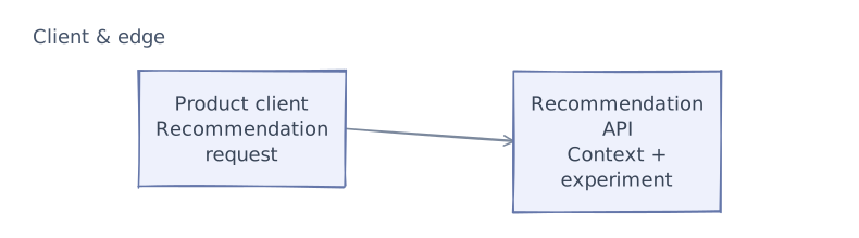
This first layer defines the system boundary. The next chapters add application logic and data dependencies. After examining the request paths and tradeoffs, we will add operational safeguards and bring the complete architecture together.
API & contracts
Phase 2 of 4 · Application & compute
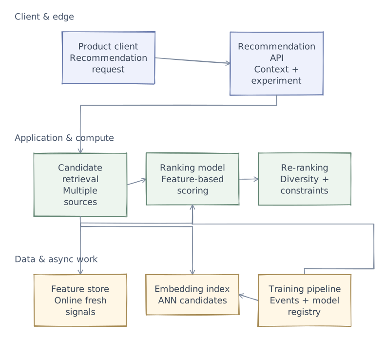
Add the application logic
Keep the entry points and add the services that do the work. Give each service a clear responsibility before defining its contracts. Storage and background dependencies come next.
- Candidate retrieval
- Retrieve a few hundred candidates from collaborative, content-based, and trending sources.
- Ranking model
- Score the candidate set using fresh features rather than evaluating the entire catalog.
- Re-ranking
- Apply eligibility, diversity, and business constraints after model scoring.
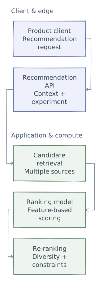
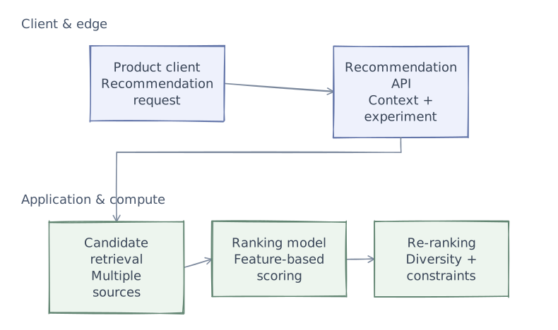
The serving request identifies the allowed user context, placement, and result limit. Return stable item IDs with enough internal trace information to connect later impressions to the recommendation decision. Keep training-only attributes out of client responses, and distinguish an empty eligible catalog from a personalization failure.
Data model
Phase 3 of 4 · Data & async work
Connect data and background work
The services now need their dependencies: durable state, fast lookups, or work that continues outside a request. Separate these responsibilities rather than treating every component as a database.
- Feature store
- Serve consistent low-latency features and manage online/offline feature skew.
- Embedding index
- Version embeddings and their index together to avoid incompatible vector spaces.
- Training pipeline
- Train on feedback with bias checks, then release models through controlled experiments.
Feature Store
Feature Architecture

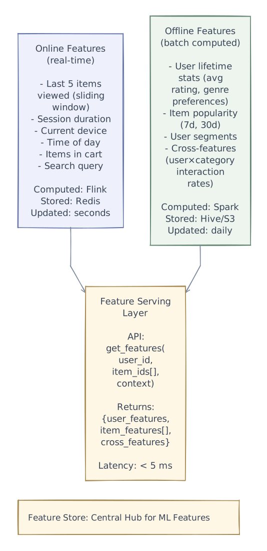
Feature Categories
| Category | Example Features | Source | Update Frequency |
|---|---|---|---|
| User static | age, gender, country, signup_date | User DB | Rarely changes |
| User behavioral | genre preferences, avg watch time, click-through rate | Batch pipeline | Daily |
| User real-time | last 5 items viewed, current session items, device | Event stream | Seconds |
| Item static | title, category, creator, price, release_date | Item DB | On item update |
| Item behavioral | popularity_7d, avg_rating, completion_rate | Batch pipeline | Daily |
| Item real-time | views_last_hour, trending_score | Event stream | Minutes |
| Cross features | user_category_affinity, user_creator_affinity | Batch pipeline | Daily |
| Context | time_of_day, day_of_week, user_location, platform | Request context | Per request |
Feature Serving Data Flow
Request arrives for user_id=42, context={mobile, evening, US}

Step 1: Fetch user features
  Redis GET user:42:features
  → {age: 28, gender: M, country: US, genre_prefs: [action:0.8, comedy:0.6],
     avg_watch_time: 45min, sessions_per_week: 12, ...}

Step 2: Fetch real-time user features
  Redis GET user:42:recent
  → {last_5_items: [item_55, item_102, item_8, item_77, item_200],
     session_items: [item_55], session_duration: 3min}

Step 3: Fetch item features (batch, for 1000 candidates)
  Redis MGET item:101:features item:102:features ... item:1100:features
  → [{category: action, popularity: 0.85, avg_rating: 4.2, ...}, ...]

Step 4: Compute cross features (on-the-fly or precomputed)
  user_42_action_affinity = 0.8 (from precomputed table)
  → Cross user×item category affinity for each candidate

Total feature fetch latency: ~3-5 ms (Redis batch reads)Core design decisions
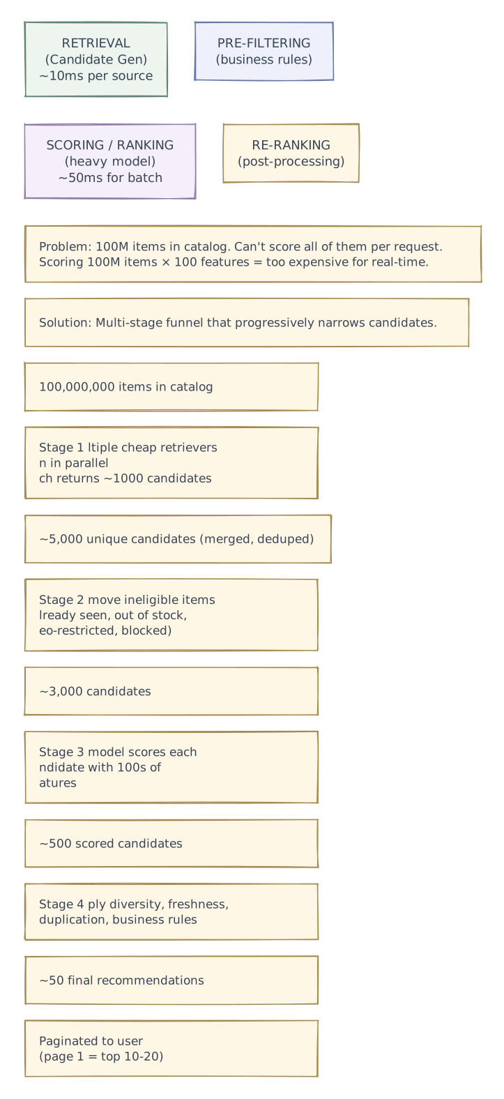
The Retrieval → Ranking Funnel
Why a Funnel?

Ranking Model
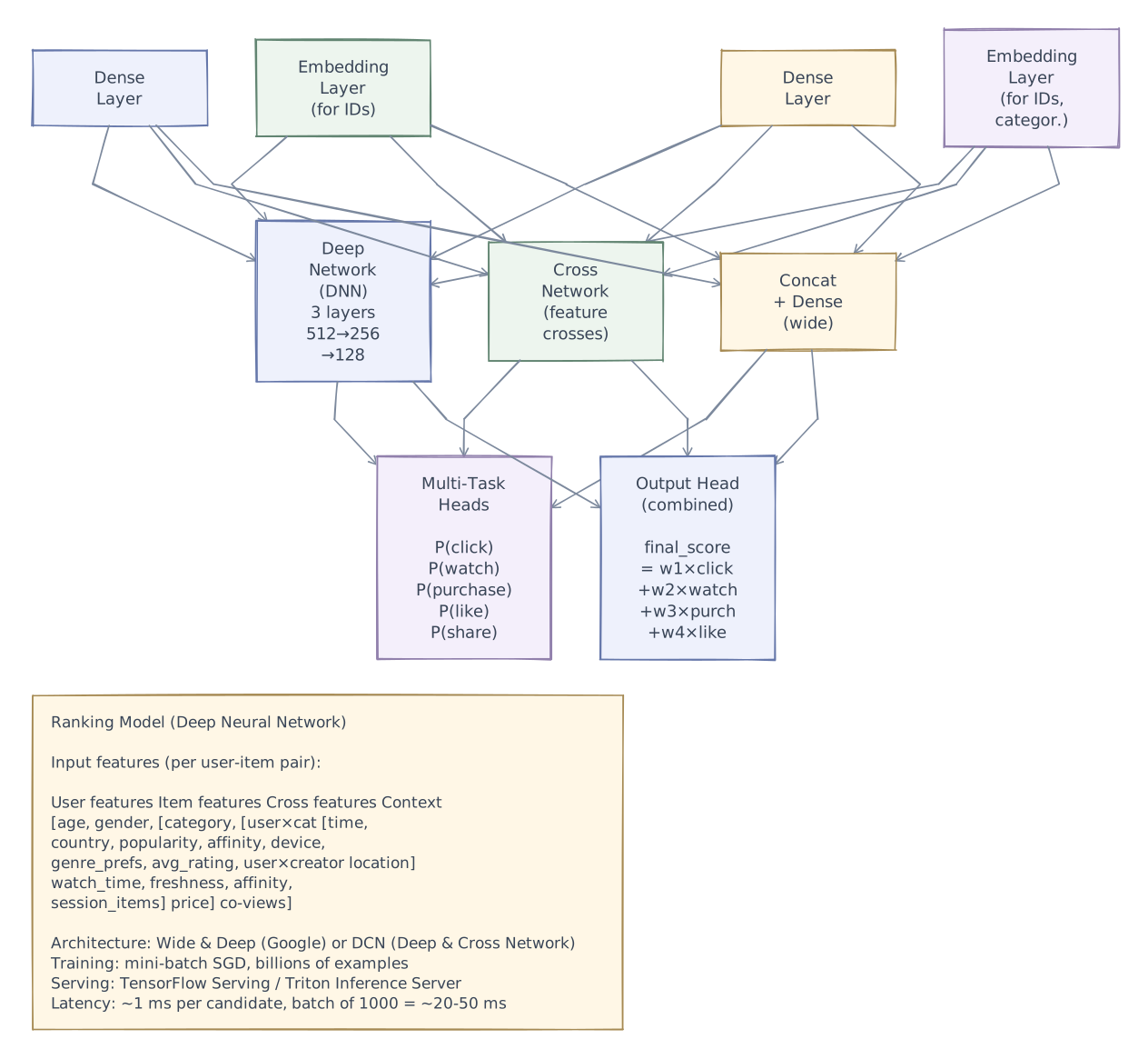
Model Architecture

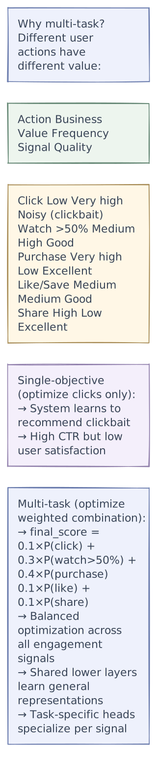
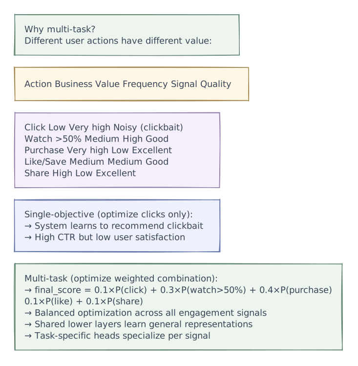
Multi-Task Learning
Ranking Score Computation
For each candidate item (1000 items per request):

1. Fetch features:
   user_features = feature_store.get_user(user_id)        // cached
   item_features = feature_store.get_items(item_ids)      // batch
   cross_features = feature_store.get_cross(user_id, item_ids)
   context = {time, device, location}

2. Batch inference:
   scores = ranking_model.predict(
     user_features,     // shared across all candidates
     item_features[],   // one per candidate
     cross_features[],  // one per candidate
     context            // shared
   )
   // Returns: [{click: 0.3, watch: 0.7, purchase: 0.05, ...}, ...]

3. Compute final score:
   for each candidate:
     final_score = 0.1 * P(click) + 0.3 * P(watch>50%)
                 + 0.4 * P(purchase) + 0.1 * P(like) + 0.1 * P(share)

4. Sort by final_score descending

Latency breakdown:
  Feature fetch:    3-5 ms
  Model inference:  20-50 ms (batched GPU)
  Sorting:          < 1 ms
  Total ranking:    ~30-55 ms
Re-Ranking & Post-Processing
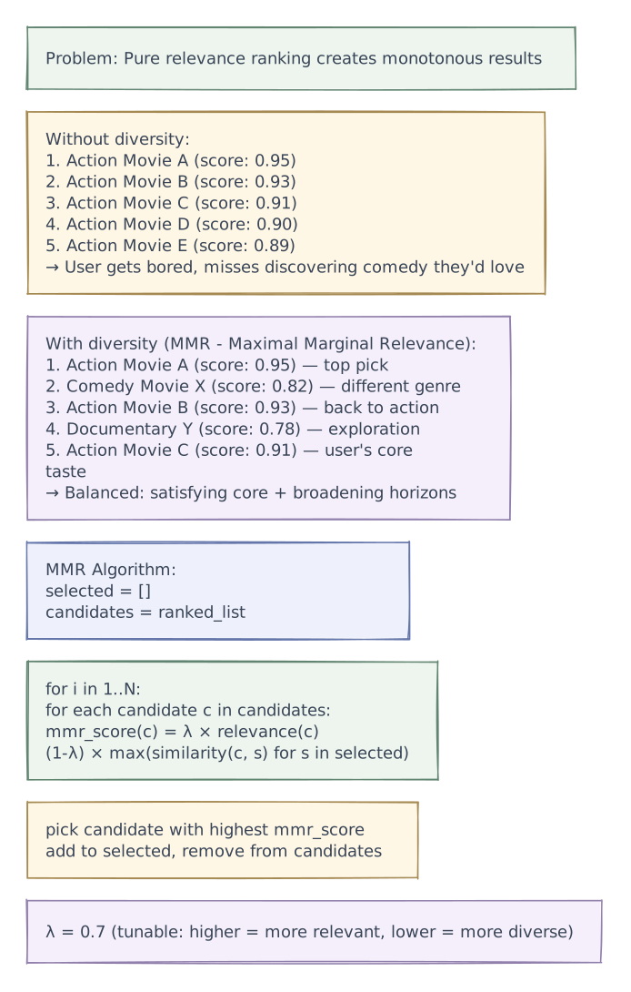
Diversity Enforcement

Business Rules & Filtering
Post-ranking filters applied in order:

1. ALREADY SEEN filter
   Remove items user has already interacted with (viewed, purchased)
   Source: user interaction history (Redis set)

2. BLOCKED / NOT INTERESTED filter
   Remove items user explicitly dismissed
   Source: user negative feedback store

3. CONTENT POLICY filter
   Remove age-restricted, geo-restricted, or policy-violating items
   Source: content moderation service

4. FRESHNESS boost
   Boost score of new items (< 7 days old) by 1.2x
   Ensures new content gets discovery opportunities

5. CREATOR DIVERSITY
   No more than 2 items from same creator in top 10
   Prevents single creator dominating recommendations

6. CATEGORY DIVERSITY
   Ensure at least 3 different categories in top 10
   Uses MMR or round-robin across category buckets

7. SPONSORED ITEMS insertion
   Insert ad/sponsored items at fixed positions (3, 7, 12)
   Only if relevance score above minimum threshold

8. EXPLANATION attachment
   For each recommended item, attach explanation:
   "Because you watched X" or "Popular in your area"
Source: retrieval source label + feature analysisRequest flows
Model Training Pipeline
Training Data Flow

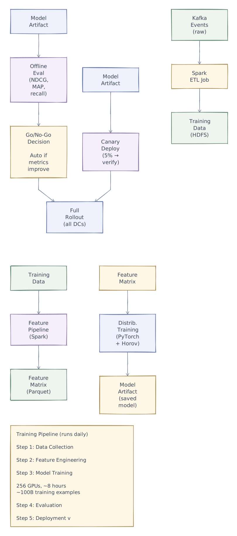
Training Data Sampling
Positive examples:
  User clicked/watched/purchased an item → (user, item, label=1)

Negative examples:
  Challenge: 100M items, user interacted with 20 → 99.99998% are "negative"
  Can't use all negatives → too imbalanced and too much data.

Negative sampling strategies:

1. Random negatives:
   Sample 5-10 random items per positive → (user, random_item, label=0)
   Simple but may include items user would never see.

2. In-batch negatives (YouTube):
   Within a training batch, treat other users' positives as negatives.
   Batch of 4096: each user's positive is negative for other 4095 users.
   Free negatives, no extra sampling needed.

3. Hard negatives:
   Items that were shown but NOT clicked → strong negative signal.
   Items retrieved but ranked low → model should learn to rank them low.
   Most informative for learning, but can bias toward popular items.

4. Mixed strategy (chosen):
   50% in-batch negatives (efficient, diverse)
   30% hard negatives (from impression logs)
20% random negatives (prevent popularity bias)Performance & caching
Retrieve a bounded candidate set before running expensive ranking features. Batch feature lookups, set deadlines for optional dependencies, and keep a non-personalized fallback ready. Cache by the context that affects eligibility, not only by user ID: an old cached recommendation must not reintroduce a removed or inaccessible item.
Advanced design
Retrieval (Candidate Generation)
Multiple Retrieval Sources

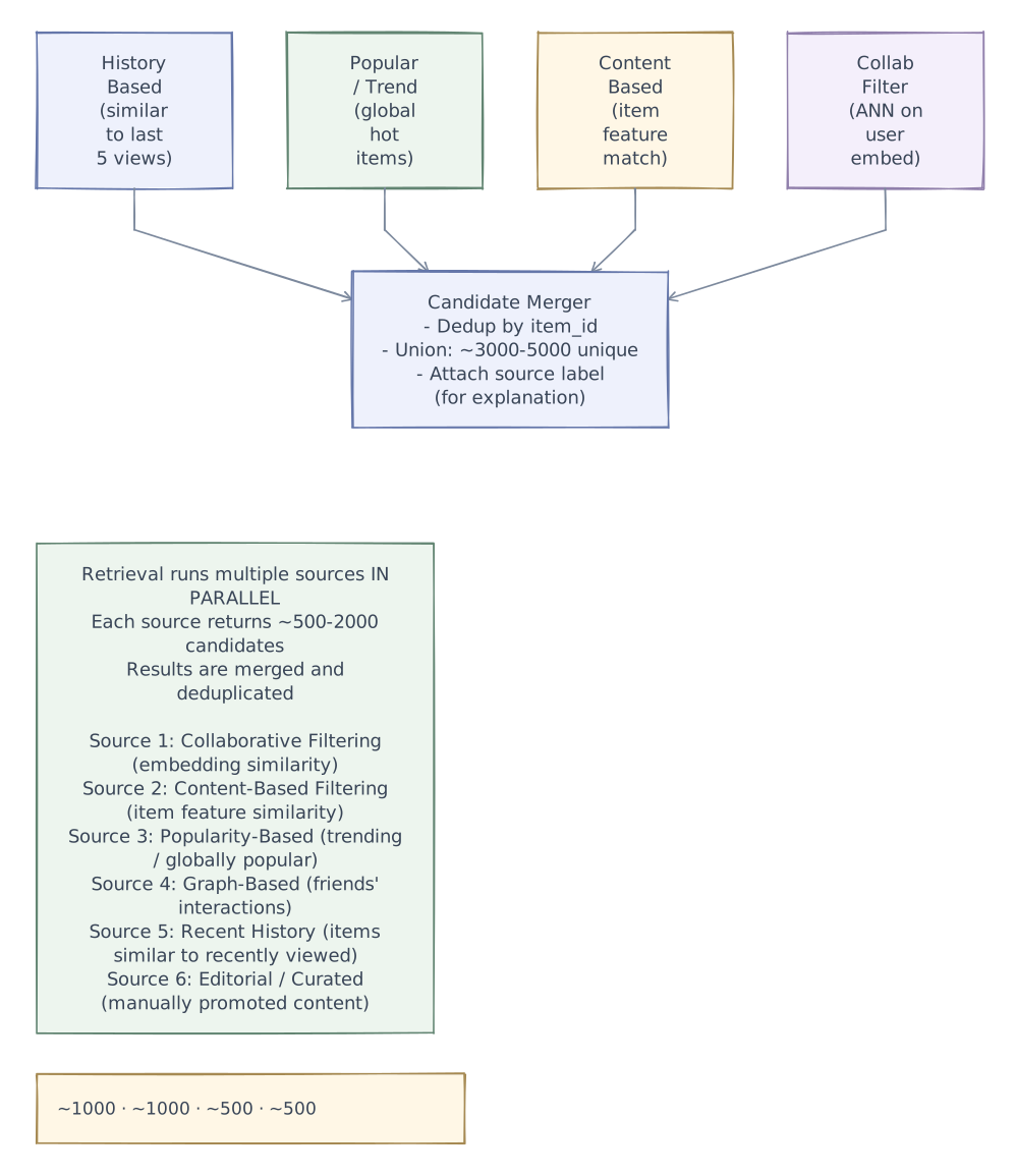
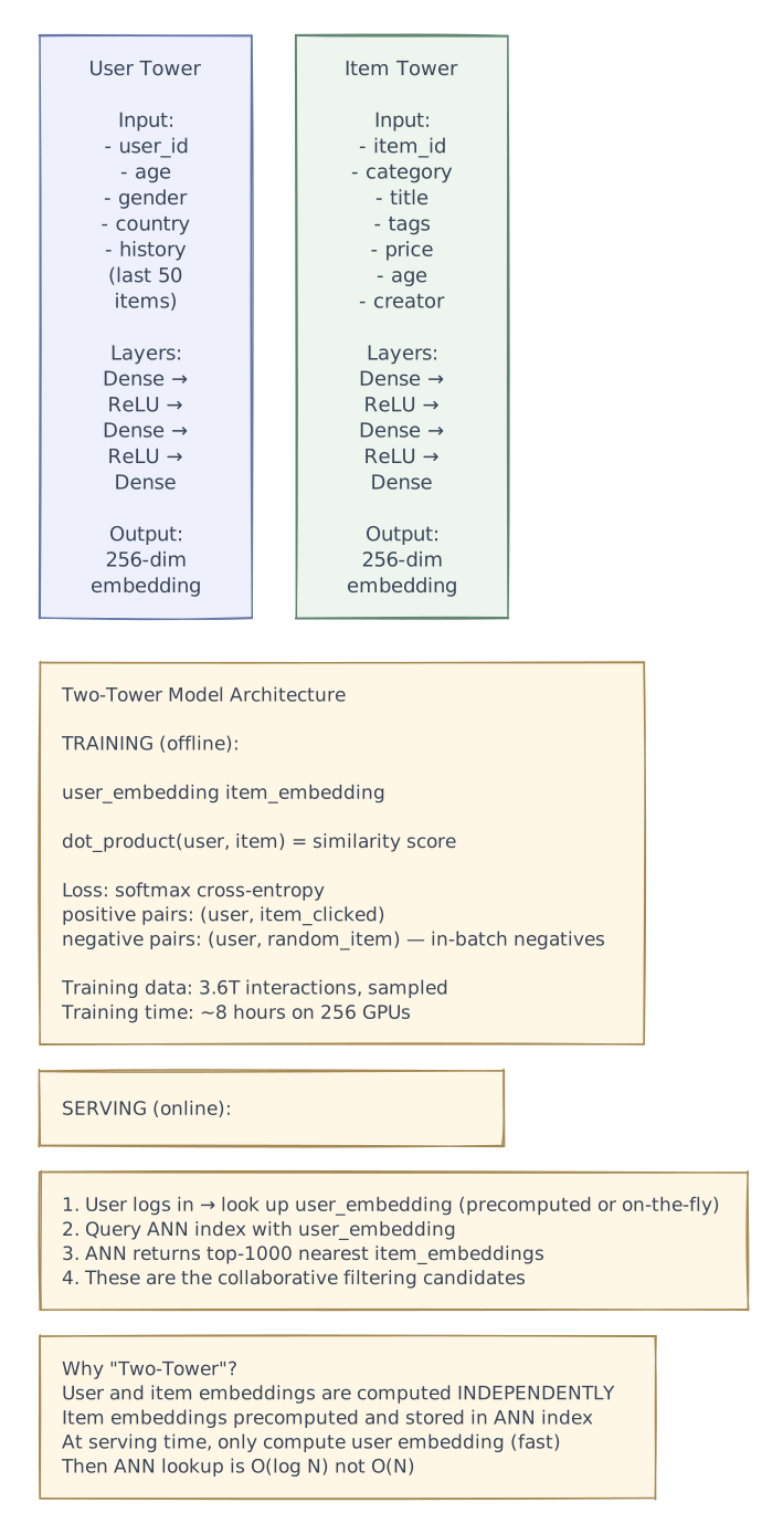
Source 1: Two-Tower Embedding Model (Primary Retrieval)

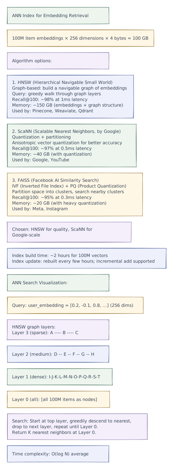
ANN (Approximate Nearest Neighbor) Index

Source 2: Content-Based Filtering

Source 3: Popularity & Trending
Simple but important retrieval source:

Global popular:
  SELECT item_id, COUNT(*) as interactions
  FROM events
  WHERE timestamp > NOW() - INTERVAL 24 HOURS
  GROUP BY item_id
  ORDER BY interactions DESC
  LIMIT 500

Segment popular (by country, age group, etc.):
  Same query but filtered by user segment.

Trending (velocity-based):
  z_score = (current_rate - historical_mean) / historical_stddev
  If z_score > 2 → item is trending

When to use:
  - Cold-start users (no history → show popular)
  - Blended with personalized results (10-20% popular items)
  - Fallback when personalization service is down
Real-Time Signal Processing
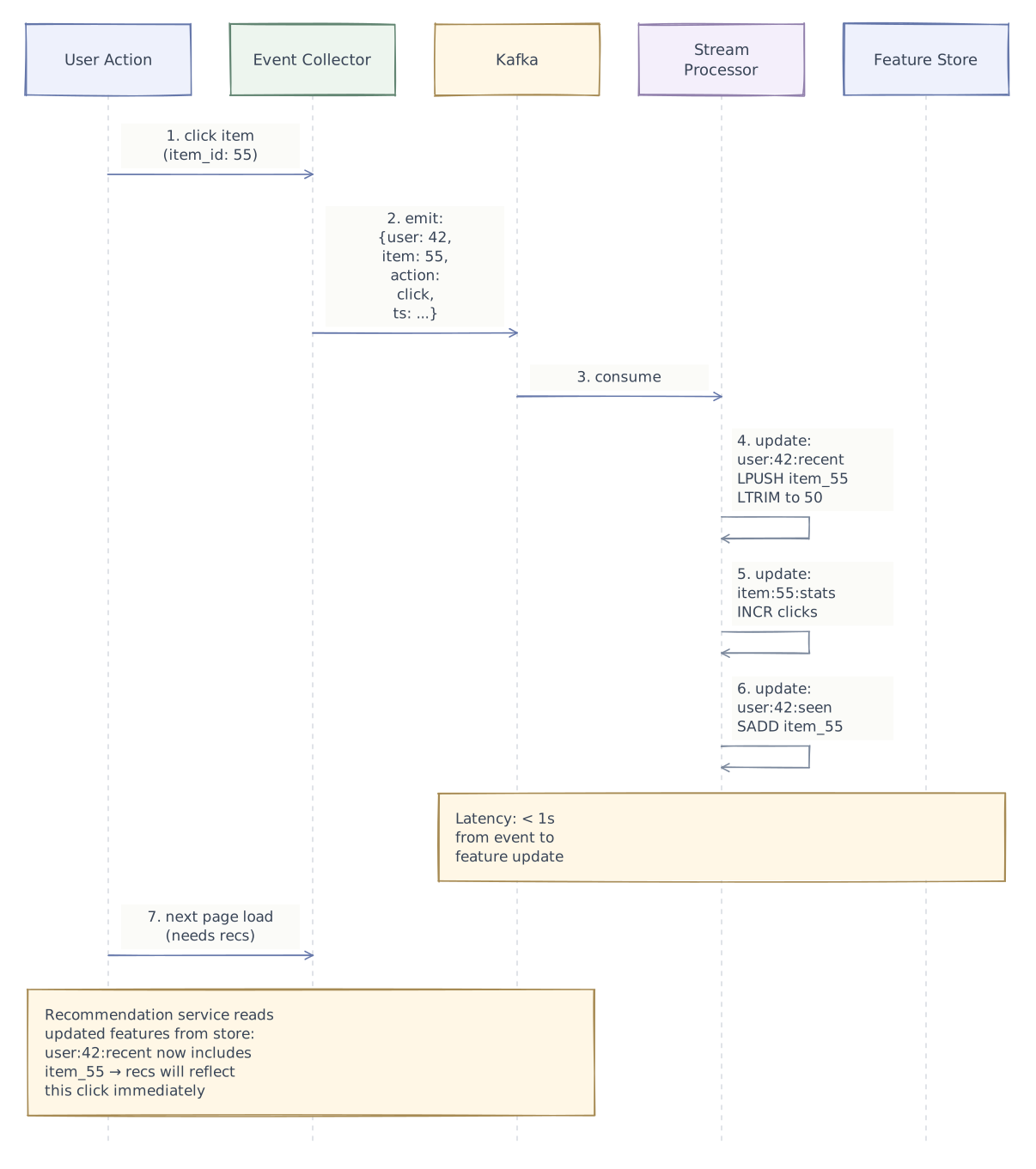
Event Processing Pipeline

Near Real-Time Embedding Updates
Problem: User embeddings from the two-tower model are trained
         offline (daily). A user who changes interest mid-day
         still sees yesterday's recommendations.

Solution: Lightweight online embedding adjustment

  1. User's base embedding: E_base (from offline model, daily)

  2. User's recent items: [item_55, item_102, item_8] (from Redis)

  3. Adjusted embedding:
     E_adjusted = α × E_base + (1-α) × mean(E_item_55, E_item_102, E_item_8)

     α = 0.7 (weight toward stable base embedding)

  4. Use E_adjusted for ANN retrieval

  This "warm-starts" from the offline embedding but shifts
  toward recent interests. Cheap to compute (just averaging).

  Full embedding retraining happens daily in batch pipeline.
A/B Testing & Experimentation
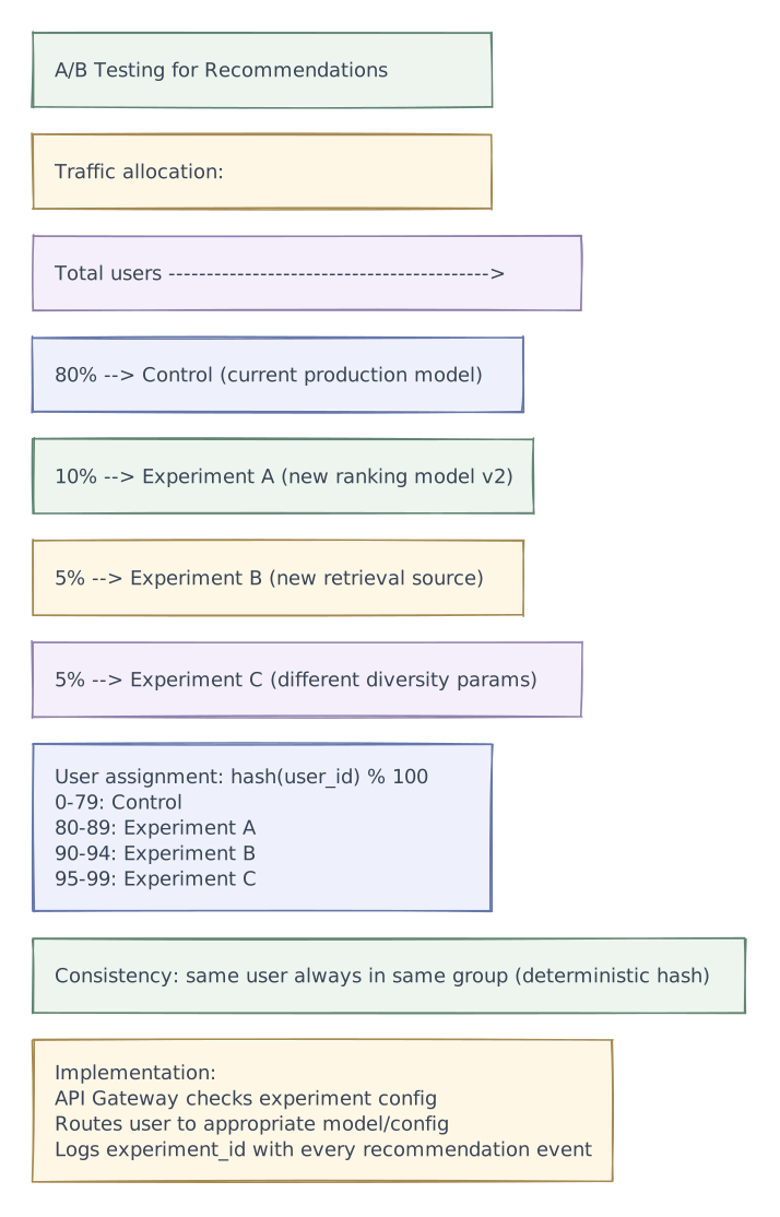
Experiment Framework

Key Metrics for A/B Testing
Guardrail metrics (must not regress):
  - DAU / MAU (user retention)
  - Revenue per user
  - Session length
  - App crashes / errors

Primary metrics (what we're trying to improve):
  - Click-through rate (CTR) on recommendations
  - Engagement rate (watch >50%, add to cart, etc.)
  - Discovery rate (% of interactions with items user hadn't seen before)
  - Long-term retention (7-day, 30-day)

Secondary metrics (nice to have):
  - Diversity of consumed content
  - Coverage (% of catalog that gets recommended)
  - Novelty (how "surprising" recommendations are)
  - Fairness (uniform exposure across item categories/creators)

Statistical significance:
  - Minimum detectable effect: 0.5% relative change
  - Required sample: ~1M users per group for 7 days
  - Significance level: p < 0.05
  - Sequential testing: monitor daily, stop early if clearly winning/losing
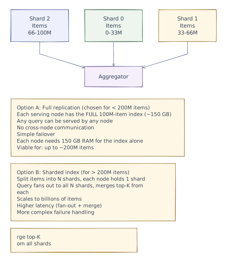
Embedding Index Management
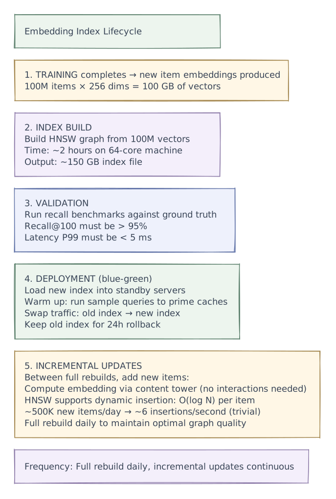
Index Lifecycle

Index Sharding vs. Replication

Edge cases
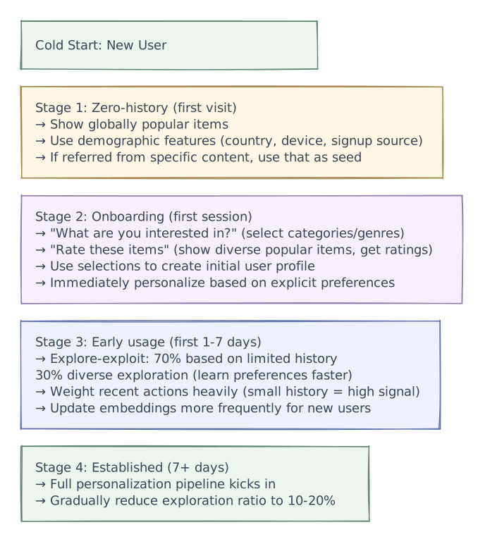
Cold Start Strategies
New User (No History)

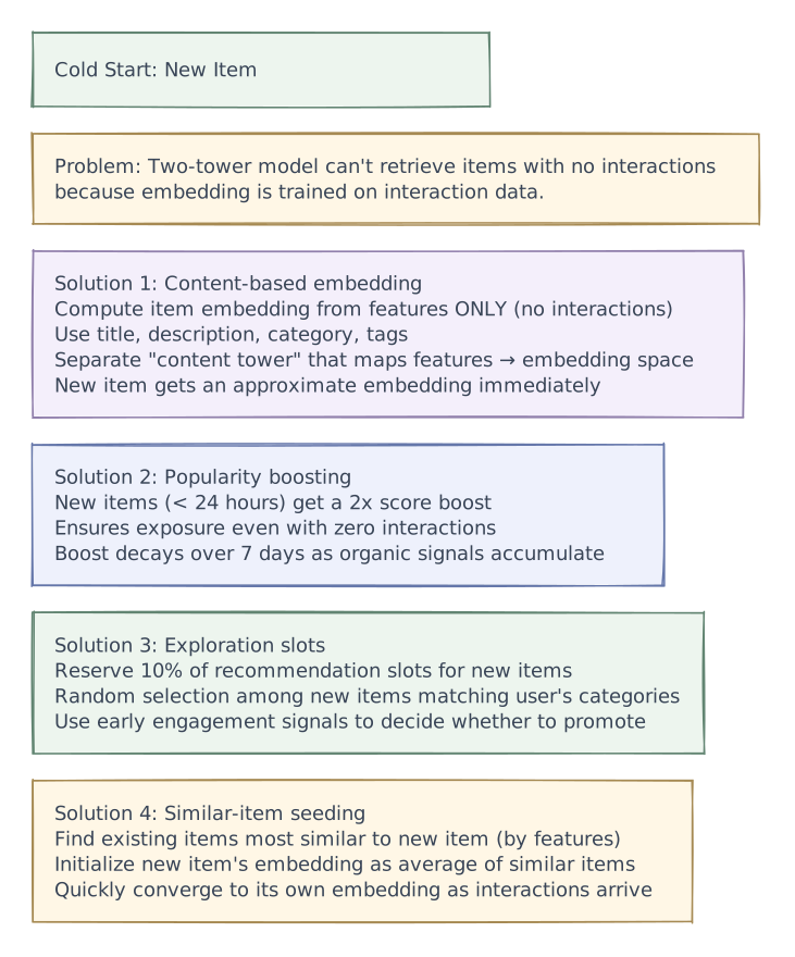
New Item (No Interactions)

Tradeoffs
Key Tradeoffs
Relevance vs. Diversity
Pure relevance optimization:
  + Highest immediate engagement (clicks, watches)
  + Users get exactly what they expect
  - Echo chamber: users never discover new interests
  - Content creator inequality (popular get richer)
  - Long-term user boredom → churn

With diversity:
  + Users discover new content → long-term engagement
  + Fairer exposure for new/niche content
  + Richer user experience
  - Lower immediate CTR on diverse items
  - Harder to measure ROI (long-term effects)

  Industry trend: optimize for LONG-TERM engagement
  not single-session metrics. Netflix found that diverse
  recommendations increase 30-day retention by ~5%.
Exploration vs. Exploitation
Exploitation (safe bets):
  Recommend items the model is confident user will like.
  High expected reward per recommendation.
  But: model never learns about uncertain items.

Exploration (discovery):
  Recommend items the model is uncertain about.
  Lower expected reward, but LEARNING value.
  Model improves faster by exploring.

Balancing strategies:

1. ε-greedy:
   90% of the time: exploit (show top-scored items)
   10% of the time: explore (show random/uncertain items)
   Simple but crude.

2. Thompson Sampling:
   Model uncertainty as probability distribution.
   Sample from distribution to decide what to show.
   Items with high uncertainty get explored naturally.
   More principled than ε-greedy.

3. Contextual Bandits:
   Full framework for explore-exploit in recommendations.
   Learn a policy that decides when to explore vs. exploit.
   State of the art but complex to implement.

Typical production choice: ε-greedy with ε=0.1-0.2
  Simple, effective, easy to tune.
Offline Training vs. Online Learning
Offline (batch) training:
  + Train on massive historical data (petabytes)
  + Stable, reproducible models
  + Easy to validate before deployment
  + GPU cluster used efficiently (full batches)
  - Model is always at least hours old
  - Can't adapt to breaking events quickly
  - Seasonal patterns require waiting for accumulation

Online (incremental) learning:
  + Adapts to new trends in minutes
  + Handles concept drift (user preferences change)
  + No need for massive retraining clusters
  - Catastrophic forgetting risk (model drifts from stable baseline)
  - Harder to debug (model changes continuously)
  - Vulnerable to data quality issues (one bad batch can corrupt model)

Hybrid (chosen):
  - Offline: full model retraining daily (stable baseline)
  - Online: lightweight feature updates in real-time (recent actions)
  - Near-online: user embedding adjustment every few minutes
  - Full online learning: reserved for specific components (e.g., CTR
    prediction head fine-tuned on last hour's data)
Pre-Computed vs. On-Demand Recommendations
Pre-computed:
  Run recommendation pipeline offline for each user.
  Store results: user_42 → [item_55, item_102, item_8, ...]
  Serve from cache/DB at request time.
  + Ultra-low latency (just a cache read)
  + No real-time compute needed
  - Stale (computed hours ago)
  - Can't incorporate request-time context (time, device, session)
  - Storage: 500M users × 200 items × 8 bytes = 800 GB

On-demand (chosen):
  Compute recommendations at request time.
  + Fresh: uses latest features and signals
  + Context-aware (time, device, session state)
  + No per-user storage needed
  - Higher serving cost (compute per request)
  - Latency depends on model complexity

Hybrid:
  Pre-compute candidates (retrieval stage, updated every few hours).
  Re-rank on demand at request time (ranking stage, real-time).
  Best of both: fast retrieval + fresh ranking.
Embedding Dimensionality
Low dimensionality (d=32-64):
  + Small ANN index (100M × 64 × 4 = 25 GB)
  + Fast ANN search
  + Less overfitting with limited data
  - Limited expressiveness (can't capture subtle preferences)

High dimensionality (d=256-512):
  + More expressive embeddings
  + Better recall for niche items
  + Captures fine-grained user preferences
  - Large ANN index (100M × 512 × 4 = 200 GB)
  - Slower ANN search
  - Requires more training data to avoid overfitting
  - Diminishing returns above ~256

Typical choice: d=128-256
  Good balance of expressiveness and efficiency.
YouTube uses 256. Spotify uses 128. Netflix uses 256.Reliability & fault tolerance
Phase 4 of 4 · Operations & resilience
Add operational safeguards
With the request paths and tradeoffs established, add the controls that help detect trouble and keep the system operating. The final diagram retains every layer introduced so far.
- Evaluation
- Monitor engagement and guardrails; serve a simpler fallback when model serving fails.

Fault Tolerance & Reliability
Failure Scenarios & Fallbacks
| Failure | Impact | Fallback |
|---|---|---|
| ANN index server down | Can't retrieve personalized candidates | Serve from other replicas; degrade to popularity-based |
| Feature store (Redis) down | Can't fetch features for ranking | Use cached features (stale); skip personalization features |
| Ranking model (GPU) down | Can't score candidates | Use lightweight model (CPU-based LambdaMART); skip neural ranking |
| Kafka event pipeline lag | Stale real-time features | Use last-known features; missing recent clicks OK for hours |
| Training pipeline fails | Stale model and embeddings | Continue serving with current model; alert ML team |
| Entire recommendation service down | No recommendations | API returns popular/trending items as emergency fallback |
Graceful Degradation Tiers
Tier 1: Full personalization (normal operation)
  Two-tower retrieval + deep ranking + real-time features + diversity
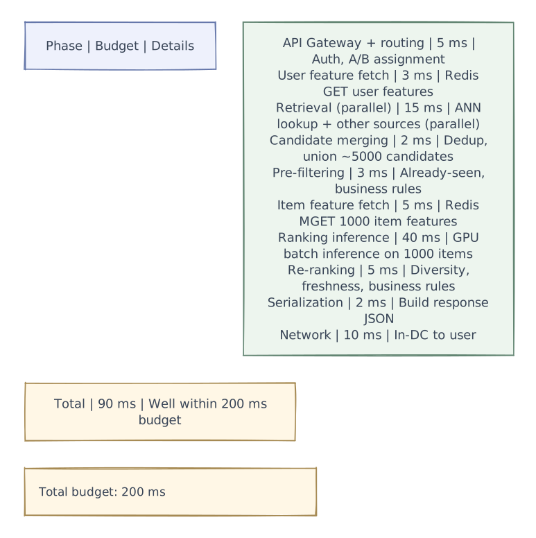
  Latency: ~90 ms

Tier 2: Simplified personalization (under stress)
  Two-tower retrieval + lightweight ranking (no GPU) + cached features
  Skip diversity re-ranking
  Latency: ~50 ms

Tier 3: Collaborative filtering only (feature store down)
  ANN retrieval on user embedding only (no features)
  Score by embedding similarity alone
  Latency: ~20 ms

Tier 4: Popularity fallback (recommendation service down)
  Return precomputed popular items by segment
  Cached in CDN/edge
  Latency: ~5 ms
Monitoring & Operational Concerns
Key Metrics
| Category | Metric | Alert Threshold |
|---|---|---|
| Latency | P50 recommendation latency | > 50 ms |
| Latency | P99 recommendation latency | > 300 ms |
| Quality | CTR on recommendations | Drop > 5% vs. previous day |
| Quality | Coverage (% of catalog recommended) | < 10% |
| Quality | Diversity (avg pairwise distance in recs) | Drop > 10% |
| Freshness | Age of newest item in recommendations | > 24 hours |
| Freshness | Model age (time since last training) | > 48 hours |
| System | ANN index recall@100 | < 93% |
| System | Feature store hit rate | < 95% |
| System | GPU utilization (ranking) | > 85% sustained |
| Pipeline | Training pipeline completion | Failure for > 2 consecutive runs |
| Pipeline | Event processing lag (Kafka) | > 5 minutes |
Debugging Recommendation Quality
When recommendation quality degrades:

1. Check model freshness
   Is the model more than 48 hours old? → Training pipeline may be broken.

2. Check feature freshness
   Are real-time features updating? → Kafka/Flink pipeline may be lagging.

3. Check ANN index
   Has recall dropped? → Index may be corrupted or stale.
   Run recall benchmark against ground truth.

4. Check traffic distribution
   Is A/B test traffic correctly routed? → Misconfigured experiment
   may be sending all users to a bad variant.

5. Check for data quality issues
   Are there spammy interactions polluting training data?
   Are there bot accounts skewing popularity signals?

6. Check coverage
   Is the system only recommending a small set of items?
   → Popularity bias may be too strong, or embedding space may have
collapsed (all items mapped to similar embeddings).Production architecture
High-Level Architecture

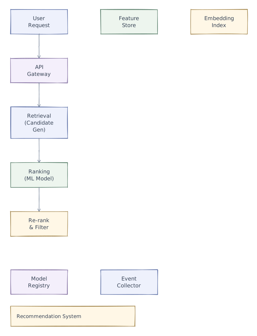
Detailed Architecture

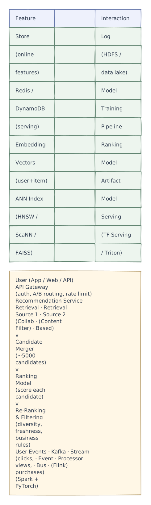
Serving Infrastructure
Global Deployment

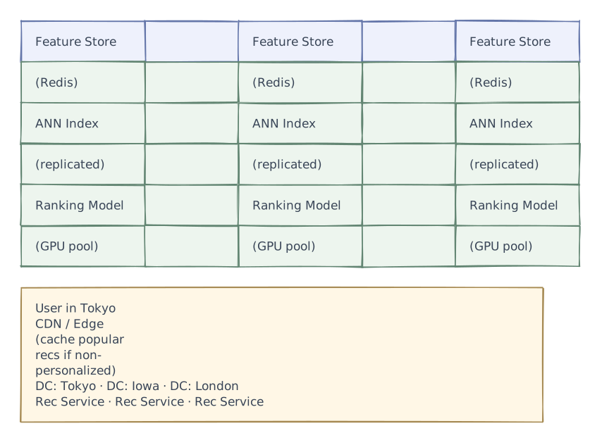
Latency Budget
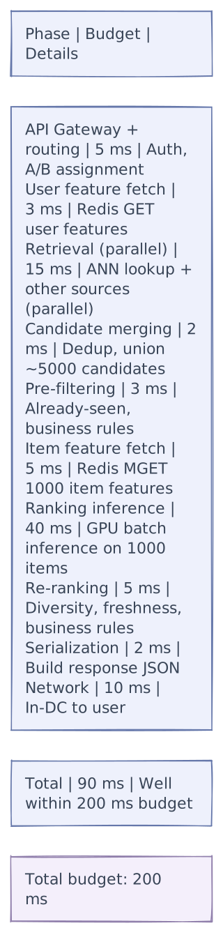
Further exploration
Handling Specific Recommendation Surfaces
"Because You Watched X" (Item-Based)
Surface: "Because you watched Inception"

Algorithm:
  1. Get embedding for "Inception": E_inception
  2. ANN search: find 20 nearest items to E_inception
  3. Filter: remove already-watched, same franchise
  4. Rank by: similarity × item_quality_score
  5. Show top 5 with explanation

  Result:
  "Because you watched Inception"
  → Tenet, Interstellar, Shutter Island, The Prestige, Memento

Implementation:
  Precomputed: For top 10K popular items, precompute similar items
  Stored in Redis: similar:item_123 → [item_456, item_789, ...]
  Updated daily when embeddings change
  For long-tail items: compute on-the-fly via ANN query
"Customers Also Bought" (Co-Purchase)
Surface: Product page, e-commerce

Algorithm: Item-Item Collaborative Filtering

  co_purchase_score(A, B) =
    |users_who_bought_both(A, B)| / sqrt(|buyers(A)| × |buyers(B)|)

  This is the cosine similarity on the purchase co-occurrence matrix.

  Precomputed:
  - Build co-purchase matrix from last 90 days of purchase data
  - For each item, store top-20 co-purchased items
  - Update daily via Spark job

  Storage: 100M items × 20 similar × 12 bytes = ~24 GB (Redis)

  Refinement:
  - Weight by recency (recent co-purchases matter more)
  - Filter out trivially co-purchased items (e.g., batteries always
    co-purchased with everything)
  - Boost complementary items (phone + case) over substitute items
    (phone + different phone)
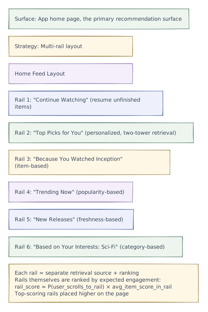
Home Feed (Personalized Mix)

Matrix Factorization (Classic Approach)
How Matrix Factorization Works
User-Item Interaction Matrix (sparse):

              Item1  Item2  Item3  Item4  Item5  ...  Item100M
  User1       5      ?      3      ?      ?
  User2       ?      4      ?      ?      2
  User3       4      ?      ?      5      ?
  User4       ?      ?      2      ?      4
  ...
  User500M    ?      3      ?      ?      ?

  ? = unknown (never interacted)
  Goal: predict the ? values

Factorization:
  R ≈ U × V^T

  R: user-item matrix (500M × 100M) — too big to store!
  U: user factor matrix (500M × k)  — k latent factors
  V: item factor matrix (100M × k)

  k = 64-256 (dimensionality of latent space)

  predicted_rating(user_i, item_j) = dot(U[i], V[j])

Training (ALS - Alternating Least Squares):
  1. Initialize U and V randomly
  2. Fix V, solve for optimal U (least squares per row)
  3. Fix U, solve for optimal V (least squares per row)
  4. Repeat until convergence (~20 iterations)

  ALS is parallelizable: each row of U/V is independent
  Run on Spark with 1000s of machines

After training:
  U[i] = user_i's embedding (what they like in latent space)
  V[j] = item_j's embedding (what it offers in latent space)

  These ARE the embeddings used for ANN retrieval!
  (Two-tower model is the deep learning evolution of this idea)
Matrix Factorization vs. Two-Tower
| Criterion | Matrix Factorization | Two-Tower Neural |
|---|---|---|
| Input | Only user-item interactions | User features + item features + interactions |
| Cold start | Poor (no embedding without interactions) | Better (features available for new items) |
| Expressiveness | Linear dot product | Non-linear deep network |
| Training | ALS (fast, parallelizable) | SGD on GPUs (slower, more compute) |
| Scale | Handles billions with ALS on Spark | Handles billions with distributed GPU training |
| Interpretability | Latent factors are opaque | Equally opaque, but feature importance available |
| State of art | Classic, still competitive | Current industry standard |
Interview playbook
System Design Interview Tips
What Interviewers Look For
- Retrieval → Ranking funnel -- this is the core architecture; explain why a funnel is necessary
- Embedding-based retrieval -- two-tower model, ANN index, how it works at scale
- Feature store -- offline vs. real-time features, how they're served
- Ranking model -- multi-task learning, feature engineering, scoring formula
- Cold start -- handling new users and new items
- Tradeoff reasoning -- relevance vs. diversity, exploration vs. exploitation, online vs. offline
Common Follow-Up Questions
| Question | Key Points |
|---|---|
| "How do you handle a new user with no history?" | Onboarding preferences → popularity → explore-exploit → full personalization |
| "How do you avoid recommending the same things?" | Already-seen filter in Redis; diversity re-ranking (MMR) |
| "What if the model starts recommending clickbait?" | Multi-task optimization (not just clicks); quality signals (watch time, shares) |
| "How do you keep recommendations fresh?" | Real-time event pipeline → feature store; incremental ANN updates; freshness boost |
| "How do you evaluate recommendation quality?" | Offline: NDCG, recall, coverage. Online: A/B test CTR, engagement, retention |
| "How does this scale to 1B users?" | Sharded feature store; replicated ANN index; stateless ranking service |
Suggested 45-Minute Interview Structure
 0-5  min:  Clarify requirements (what kind of items? scale? latency?)
 5-10 min:  Scale estimations (users, items, interactions, QPS)
10-20 min:  Retrieval → Ranking funnel (the core architecture)
20-30 min:  Deep dive: pick ONE
            - Option A: Two-tower model + ANN retrieval
            - Option B: Feature store + ranking model
            - Option C: Real-time signal processing
30-38 min:  Cold start + diversity strategies
38-43 min:  Tradeoffs (relevance vs diversity, online vs offline, embedding dims)
43-45 min:  Monitoring, A/B testing, failure handling